Earthquake Report: Lombok, Indonesia

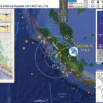
Earlier today there was a shallow M 6.4 earthquake with an epicenter on the island of Lombok, Indonesia. With a hypocentral depth of about 7.5 km, this size of an earthquake can be quite damaging. The USGS PAGER estimate of impact suggests that there is about a 10% chance that there are more than 10 fatalities. Hopefully there are none. There have been several aftershocks, two M > 5.

This earthquake is probably along a thrust fault associated with the Flores thrust fault, a north vergent (dipping into the earth in a southerly direction) back thrust fault to the Sunda subduction zone fault. The Flores thrust possibly extends from east of Timor on the east to the northern shore of Java (McCaffrey and Nabelek, 1987). Others suggest that the Flores thrust ends at a cross fault just east of Lombok (Hengresh and Whitney, 2016). However, the seismic profiles from Silver et al. (1986) are convincing that there are east-west compressional structures extending between the northern shore of Java to where the Flores thrust is mapped.

Detailed mapping of the seafloor to the east of Lombok, north of the island of Sumbawa, reveals that there are imbricate (overlapping) thrust faults (Silver et al., 1986). I think that it is reasonable to presume that there are similar structures on the northern flank of Lombok.

Lombok is also a volcano complex as part of the Sunda magmatic arc. There may be fault systems associated with the volcanic activity. I include tectonic faults that are included in the global scale fault data set from the Coordinating Committee for Geoscience Programme in East and Southeast Asia. The most active volcano on Lombok is the Rinjani volcano. Here is a great place to learn about this volcano (the Volcano Discovery website).

If the M 6.4 earthquake was on the Flores fault, it would need to dip at about 10°. The Flores thrust fault proposed by Hengesh and Whitney (2016) has a much steeper dip. So this sequence is probably in the upper plate somewhere.

There was a M 6.0 earthquake to the east of the M 6.4, but it was much deeper (almost 600 km), so is unlikely to be genetically related to the M 6.4 sequence.

Magnetic Anomalies

  • In the map below, I include a transparent overlay of the magnetic anomaly data from EMAG2 (Meyer et al., 2017). As oceanic crust is formed, it inherits the magnetic field at the time. At different points through time, the magnetic polarity (north vs. south) flips, the north pole becomes the south pole. These changes in polarity can be seen when measuring the magnetic field above oceanic plates. This is one of the fundamental evidences for plate spreading at oceanic spreading ridges (like the Gorda rise).
  • Regions with magnetic fields aligned like today’s magnetic polarity are colored red in the EMAG2 data, while reversed polarity regions are colored blue. Regions of intermediate magnetic field are colored light purple.
  • We can see the roughly east-west trends of these red and blue stripes. These lines are parallel to the ocean spreading ridges from where they were formed. The stripes disappear at the subduction zone because the oceanic crust with these anomalies is diving deep beneath the Sunda plate (part of Eurasia), so the magnetic anomalies from the overlying Sunda plate mask the evidence for the Australia plate.

Historic Seismicity

  • Below I discuss analogues to today’s M 6.4 earthquake.
  • To the west, between Lombok and Bali, there was a series of earthquakes all in 1979. They happened several months apart, but had a similar magnitude and orientation. The hypocentral depths were in the 25-40 km depth range, so some of these may have been on the Flores thrust system. These alone suggest that the Flores thrust extends at least this far west.
  • To the east, along the eastern part of Sumbawa, there was a series of earthquakes in the first decade of the 21st century, from 2002-2009. These also all share a similar magnitude range and orientation. These earthquakes all happened within a narrow range of depths (18-20 km; though the 2002 earthquake has a default depth on 10 km).
  • Based on earthquakes in the regions to the east and to the west, it is possible that this M 6.4 is the first of a series of mid M 6 earthquakes (either within a year like in Bali or over several years like Sumbawa).

Below is my interpretive poster for this earthquake

I plot the seismicity from the past month, with color representing depth and diameter representing magnitude (see legend). I include earthquake epicenters from 1918-2018 with magnitudes M ≥ 6.0.
I plot the USGS fault plane solutions (moment tensors in blue and focal mechanisms in orange), possibly in addition to some relevant historic earthquakes.

  • I placed a moment tensor / focal mechanism legend on the poster. There is more material from the USGS web sites about moment tensors and focal mechanisms (the beach ball symbols). Both moment tensors and focal mechanisms are solutions to seismologic data that reveal two possible interpretations for fault orientation and sense of motion. One must use other information, like the regional tectonics, to interpret which of the two possibilities is more likely.
  • I also include the shaking intensity contours on the map. These use the Modified Mercalli Intensity Scale (MMI; see the legend on the map). This is based upon a computer model estimate of ground motions, different from the “Did You Feel It?” estimate of ground motions that is actually based on real observations. The MMI is a qualitative measure of shaking intensity. More on the MMI scale can be found here and here. This is based upon a computer model estimate of ground motions, different from the “Did You Feel It?” estimate of ground motions that is actually based on real observations.
  • I include the slab contours plotted (Hayes et al., 2012), which are contours that represent the depth to the subduction zone fault. These are mostly based upon seismicity. The depths of the earthquakes have considerable error and do not all occur along the subduction zone faults, so these slab contours are simply the best estimate for the location of the fault.
  • I include some inset figures.

  • In the upper right corner is a low angle oblique view of the Sunda subduction zone beneath Java, Bali, Lombok, and Sumbawa (from Earth Observatory Singapore). I place a blue star in the general location of today’s earthquake’s epicenter (as for all figures here). The India-Australia plate is subducting northwards beneath the Sunda plate (part of the Eurasia plate).
  • In the upper left corner is a plate tectonic map showing the major fault systems, volcanic arc islands, and oceanic plateaus and basins of the region (Darman, 2012). The map shows the Flores thrust extending as far west as Lombok. Compare the complicated tectonics in the eastern portion of this region compared to the western portion of this region.
  • To the right of the Darman (2012) map is a cross section of seismicity presented by Hengresh and Whitney (2016). These authors argue for a north vergent Flores thrust in this region, though most of their work was on the subduction/collision zone.
  • In the lower right corner is another, earlier, tectonic map from Silver et al. (1986). These authors use seismic reflection and multibeam bathymetry data to map the Flores thrust as far as Java, west of Bali. The location for the map in the lower left corner of this interpretive poster is outlined here as a dashed line rectangle.
  • In the lower left corner is a map from Silver et al. (1986) that shows the detailed mapping of imbricate north (and some south) vergent thrust faults.
  • Here is the same map but with seismicity from the past month.


  • Here is the same map but with historic seismicity.


USGS Earthquake Pages

    These are from this current sequence

  • 2018-07-28 17:07:23 UTC M 6.0
  • 2018-07-28 22:47:37 UTC M 6.4
  • 2018-07-28 23:06:49 UTC M 5.4
  • 2018-07-29 01:50:32 UTC M 5.3

Other Report Pages

Some Relevant Discussion and Figures

  • Below is a map showing historic seismicity (Jones et al., 2014). Cross sections B-B’ and C-C’ are shown. The seismicity for the cross sections below are sourced from within each respective rectangle.

  • Here are the seismcity cross sections.

  • Here is the map from McCaffrey and Nabelek (1987). They used seismic reflection profiles, gravity modeling along these profiles, seismicity, and earthquake source mechanism analyses to support their interpretations of the structures in this region.

  • Tectonic and geographic map of the eastern Sunda arc and vicinity. Active volcanoes are represented by triangles, and bathymetric contours are in kilometers. Thrust faults are shown with teeth on the upper plate. The dashed box encloses the study area.

  • Here is the Audley (2011) cross section showing how the backthrust relates to the subduction zone beneath Timor. I include their figure caption in blockquote below.

  • Cartoon cross section of Timor today, (cf. Richardson & Blundell 1996, their BIRPS figs 3b, 4b & 7; and their fig. 6 gravity model 2 after Woodside et al. 1989; and Snyder et al. 1996 their fig. 6a). Dimensions of the filled 40 km deep present-day Timor Tectonic Collision Zone are based on BIRPS seismic, earthquake seismicity and gravity data all re-interpreted here from Richardson & Blundell (1996) and from Snyder et al. (1996). NB. The Bobonaro Melange, its broken formation and other facies are not indicated, but they are included with the Gondwana mega-sequence. Note defunct Banda Trench, now the Timor TCZ, filled with Australian continental crust and Asian nappes that occupy all space between Wetar Suture and the 2–3 km deep deformation front north of the axis of the Timor Trough. Note the much younger decollement D5 used exactly the same part of the Jurassic lithology of the Gondwana mega-sequence in the older D1 decollement that produced what appears to be much stronger deformation.

  • This are the seismicity cross sections from Hangesh and Whitney (2016). These are shown to compare the subduction zone offshore of Java and the collision zone in the Timor region.

  • Comparison of hypocentral profiles across the (a) Java subduction zone and (b) Timor collision zone (paleo-Banda trench). Catalog compiled from multiple reporting agencies listed in Table 1. Events of Mw>4.0 are shown for period 1815 to 2015.

  • Here is a map of the same general area from Silver et al. (1986), used here to locate the following large scale map.

  • Location of SeaMARC II survey (Plate 1 and Figures 2) and geographic features discussed in text. Triangles on upper plates of thrust zones.

  • This is the large scale map showing the detailed thrust fault mapping (Silver et al., 1986).

  • Bathymetry, faults, and mud diapirs of the central Flores thrust zone, based on interpretation of SeaMARC II data and seismic reflection profiles. Shown also are locations (circled numbers) of all seismic profiles. Mud diapirs are solid black. Triangles on upper plates of thrust faults.

  • Here is the tectonic map from Hangesh and Whitney (2016).

  • Illustration of major tectonic elements in triple junction geometry: tectonic features labeled per Figure 1; seismicity from ISC-GEM catalog [Storchak et al., 2013]; faults in Savu basin from Rigg and Hall [2011] and Harris et al. [2009]. Purple line is edge of Australian continental basement and fore arc [Rigg and Hall, 2011]. Abbreviations: AR = Ashmore Reef; SR = Scott Reef; RS = Rowley Shoals; TCZ = Timor Collision Zone; ST = Savu thrust; SB = Savu Basin; TT = Timor thrust; WT =Wetar thrust; WASZ = Western Australia Shear Zone. Open arrows indicate relative direction of motion; solid arrows direction of vergence.

  • Here are some focal mechanisms from earthquakes in the region from Hangesh and Whitney (2016). Symbol color represents depth.

  • (a) Focal mechanism solutions for the study region. The focal mechanisms are classified based on depth intervals to illustrate the style of faulting within the different structural domains. Note (b) sinistral reverse motion along Timor trough, (c) subduction related pattern along Java trench, and dextral solutions along the western Australia extended margin (Figure 4a) north of 20°S. Centroid moment tensor (CMT) solutions [Dziewonski et al., 1981] are from the CMT project [Ekström et al., 2012; http://www.globalcmt.org/CMTcite.html] for events of Mw>5.0 for the period 1976 onward.

  • Here is a figure showing the regional geodetic motions (Bock et al., 2003). I include their figure caption below as a blockquote.

  • Topographic and tectonic map of the Indonesian archipelago and surrounding region. Labeled, shaded arrows show motion (NUVEL-1A model) of the first-named tectonic plate relative to the second. Solid arrows are velocity vectors derived from GPS surveys from 1991 through 2001, in ITRF2000. For clarity, only a few of the vectors for Sumatra are included. The detailed velocity field for Sumatra is shown in Figure 5. Velocity vector ellipses indicate 2-D 95% confidence levels based on the formal (white noise only) uncertainty estimates. NGT, New Guinea Trench; NST, North Sulawesi Trench; SF, Sumatran Fault; TAF, Tarera-Aiduna Fault. Bathymetry [Smith and Sandwell, 1997] in this and all subsequent figures contoured at 2 km intervals.

  • This map from Hangesh and Whitney (2016) shows the GPS velocities in this region. Note the termination of the Flores thrust and the north-northeast striking (oriented) cross fault between Lombok and Sumbawa.

  • GPS velocities of Sunda and Banda arc region. Large black and grey arrow shows motion of Australia relative to Eurasia [DeMets et al., 1994]. Thin black arrows show GPS velocities of Sunda and Banda arc regions relative to Australia [Nugroho et al., 2009]. Seismicity from ISC-GEM catalog [Storchak et al., 2013]. Note reduction of station velocities from west to east indicating progressive coupling of the Banda arc to the Australian plate compared to the area along the Sunda arc.

Geologic Fundamentals

  • For more on the graphical representation of moment tensors and focal mechnisms, check this IRIS video out:
  • Here is a fantastic infographic from Frisch et al. (2011). This figure shows some examples of earthquakes in different plate tectonic settings, and what their fault plane solutions are. There is a cross section showing these focal mechanisms for a thrust or reverse earthquake. The upper right corner includes my favorite figure of all time. This shows the first motion (up or down) for each of the four quadrants. This figure also shows how the amplitude of the seismic waves are greatest (generally) in the middle of the quadrant and decrease to zero at the nodal planes (the boundary of each quadrant).

  • There are three types of earthquakes, strike-slip, compressional (reverse or thrust, depending upon the dip of the fault), and extensional (normal). Here is are some animations of these three types of earthquake faults. The following three animations are from IRIS.
  • Strike Slip:

    Compressional:

    Extensional:

  • This is an image from the USGS that shows how, when an oceanic plate moves over a hotspot, the volcanoes formed over the hotspot form a series of volcanoes that increase in age in the direction of plate motion. The presumption is that the hotspot is stable and stays in one location. Torsvik et al. (2017) use various methods to evaluate why this is a false presumption for the Hawaii Hotspot.

  • A cutaway view along the Hawaiian island chain showing the inferred mantle plume that has fed the Hawaiian hot spot on the overriding Pacific Plate. The geologic ages of the oldest volcano on each island (Ma = millions of years ago) are progressively older to the northwest, consistent with the hot spot model for the origin of the Hawaiian Ridge-Emperor Seamount Chain. (Modified from image of Joel E. Robinson, USGS, in “This Dynamic Planet” map of Simkin and others, 2006.)

  • Here is a map from Torsvik et al. (2017) that shows the age of volcanic rocks at different locations along the Hawaii-Emperor Seamount Chain.

  • Hawaiian-Emperor Chain. White dots are the locations of radiometrically dated seamounts, atolls and islands, based on compilations of Doubrovine et al. and O’Connor et al. Features encircled with larger white circles are discussed in the text and Fig. 2. Marine gravity anomaly map is from Sandwell and Smith.

    References:

  • Audley-Charles, M.G., 1986. Rates of Neogene and Quaternary tectonic movements in the Southern Banda Arc based on micropalaeontology in: Journal of fhe Geological Society, London, Vol. 143, 1986, pp. 161-175.
  • Audley-Charles, M.G., 2011. Tectonic post-collision processes in Timor, Hall, R., Cottam, M. A. &Wilson, M. E. J. (eds) The SE Asian Gateway: History and Tectonics of the Australia–Asia Collision. Geological Society, London, Special Publications, 355, 241–266.
  • Baldwin, S.L., Fitzgerald, P.G., and Webb, L.E., 2012. Tectonics of the New Guinea Region in Annu. Rev. Earth Planet. Sci., v. 41, p. 485-520.
  • Benz, H.M., Herman, Matthew, Tarr, A.C., Hayes, G.P., Furlong, K.P., Villaseñor, Antonio, Dart, R.L., and Rhea, Susan, 2011. Seismicity of the Earth 1900–2010 New Guinea and vicinity: U.S. Geological Survey Open-File Report 2010–1083-H, scale 1:8,000,000.
  • Darman, H., 2012. Seismic Expression of Tectonic Features in the Lesser Sunda Islands, Indonesia in Berita Sedimentologi, Indonesian Journal of Sedimentary Geology, no. 25, po. 16-25.
  • Hall, R., 2011. Australia-SE Asia collision: plate tectonics and crustal flow in Geological Society, London, Special Publications 2011; v. 355; p. 75-109 doi: 10.1144/SP355.5
  • Hangesh, J. and Whitney, B., 2014. Quaternary Reactivation of Australia’s Western Passive Margin: Inception of a New Plate Boundary? in: 5th International INQUA Meeting on Paleoseismology, Active Tectonics and Archeoseismology (PATA), 21-27 September 2014, Busan, Korea, 4 pp.
  • Hayes, G.P., Wald, D.J., and Johnson, R.L., 2012. Slab1.0: A three-dimensional model of global subduction zone geometries in, J. Geophys. Res., 117, B01302, doi:10.1029/2011JB008524
  • Jones, E.S., Hayes, G.P., Bernardino, Melissa, Dannemann, F.K., Furlong, K.P., Benz, H.M., and Villaseñor, Antonio, 2014. Seismicity of the Earth 1900–2012 Java and vicinity: U.S. Geological Survey Open-File Report 2010–1083-N, 1 sheet, scale 1:5,000,000, https://dx.doi.org/10.3133/ofr20101083N.
  • McCaffrey, R., and Nabelek, J.L., 1984. The geometry of back arc thrusting along the Eastern Sunda Arc, Indonesia: Constraints from earthquake and gravity data in JGR, Atm., vol., 925, no. B1, p. 441-4620, DOI: 10.1029/JB089iB07p06171
  • Okal, E. A., & Reymond, D., 2003. The mechanism of great Banda Sea earthquake of 1 February 1938: applying the method of preliminary determination of focal mechanism to a historical event in EPSL, v. 216, p. 1-15.
  • Silver, E.A., Breen, N.A., and Prastyo, H., 1986. Multibeam Study of the Flores Backarc Thrust Belt, Indonesia, in JGR., vol. 91, no. B3, p. 3489-3500
  • Zahirovic, S., Seton, M., and Müller, R.D., 2014. The Cretaceous and Cenozoic tectonic evolution of Southeast Asia in Solid Earth, v. 5, p. 227-273, doi:10.5194/se-5-227-2014

Earthquake Report: Madagascar!

Today there was an earthquake in a region that we don’t hear about that often. Madagascar is off the coast of southeastern Africa and the oceanic basin to the west is likely formed as part of the East Africa Rift system, but also due to the post Gondwana plate tectonics. Madagascar was once part of India, back when India was part of Gondwana.
Today’s (and of the last few days) earthquakes are located along the Comoros Archipelago, volcanic islands formed from hotspot volcanism.
There exist fracture zones in this region. Below, we see that these fracture zones have been interpreted as right-lateral strike-slip faults. However, the relative offsets of magnetic anomalies (and spreading ridges) show that these faults are instead left-lateral. So, that is my interpretation for this M 5.8 earthquake, a left-lateral strike-slip earthquake. I placed white dashed lines in the poster below to show where some of these fracture zones may be located, based upon the magnetic anomaly data (EMAG2).

Below is my interpretive poster for this earthquake

I plot the seismicity from the past month, with color representing depth and diameter representing magnitude (see legend). I include earthquake epicenters from 1918-2018 with magnitudes M ≥ 4.5.
I plot the USGS fault plane solutions (moment tensors in blue and focal mechanisms in orange) for the M 5.8 earthquake.

  • I placed a moment tensor / focal mechanism legend on the poster. There is more material from the USGS web sites about moment tensors and focal mechanisms (the beach ball symbols). Both moment tensors and focal mechanisms are solutions to seismologic data that reveal two possible interpretations for fault orientation and sense of motion. One must use other information, like the regional tectonics, to interpret which of the two possibilities is more likely.
  • I also include the shaking intensity contours on the map. These use the Modified Mercalli Intensity Scale (MMI; see the legend on the map). This is based upon a computer model estimate of ground motions, different from the “Did You Feel It?” estimate of ground motions that is actually based on real observations. The MMI is a qualitative measure of shaking intensity. More on the MMI scale can be found here and here. This is based upon a computer model estimate of ground motions, different from the “Did You Feel It?” estimate of ground motions that is actually based on real observations.
  • I include some inset figures.

  • In the upper center right is a figure from James Wood and Alex Guth, showing the rift systems in eastern Africa.
  • In the upper left corner is a figure showing the estimated (reconstructed) location of Madagascar within Gondwana (Reeves, 2014).
  • In the lower left corner is a map that shows the East Africa Rift system, along with the offshore branch (associated with the Davie fracture zone). The M 5.8 earthquake is just to the east of the larger scale map (Franke et al., 2015).
  • In the upper right corner is a figure that shows a reconstruction of the position of Madagascar (Phethean et al., 2017). The blue lines are pathway lines showing how Madagascar moved away from Africa. Spreading ridges are shown in red. The offsets of the spreading ridges show left lateral strike slip offsets of these ridges.
  • In the lower right corner is a map that shows the free-air gravity data that Phethean et al. (2017) used to make their reconstruction. Note that they interpret these faults as right lateral strike-slip. This interpretation is in contrast to the relative offsets of the oceanic spreading ridges. I placed a blue star in the general location of today’s M 5.8 earthquake.


USGS Earthquake Pages

Some Relevant Discussion and Figures

  • Here is the plate reconstruction figure from Phethean et al. (2017).

  • Plate tectonic reconstruction of Madagascar’s escape from Africa from the Early Jurassic to the cessation of spreading in the Cretaceous. Madagascar is shown without the remainder of East Gondwana (India, Antarctica, and Australia) attached. (a) Present-day sediment thickness in the Western Somali Basin taken from the CRUST1.0 model. (b–e) The key stages of Madagascar’s motion out of Africa. Modeled flow lines are shown as blue-arrowed lines where the center of symmetry is marked by orange circles. (f) Madagascar’s present-day position, which is reached at around 125 Ma. Flow lines closely match the fracture zone pattern of the basin (additional black lines), and the basin’s predicted final symmetry (orange circles) lies in good agreement with the interpreted extinct mid-ocean ridge system (red lines). Locations of magnetic anomalies used to temporally constrain plate motions shown with symbols as interpreted by Davis et al. [2016].

  • Here is the summary figure, showing their interpretation of the different fracture zones (Phethean et al., 2017).

  • (a) Commonly interpreted basin configuration, where the continent-ocean transition is assumed to follow the DFZ [e.g., Bunce and Molnar, 1977; Coffin and Rabinowitz, 1987; Gaina et al., 2013]. (b) Schematic of the basin configuration suggested in this study, with strike-slip tectonics dominating along the edge of the Rovuma Basin, while much of the Tanzania Coastal Basin should be considered as an obliquely rifted margin. The Davie Fracture Zone is a major ocean-ocean fracture zone, not the continent-ocean transform margin. DFZ, Davie Fracture Zone; DHOW, Dhow Fracture Zone; VLCC, Very Large Crude Carrier Fracture Zone; ARS, Auxiliary Rescue and Salvage Fracture Zone. (c) Free-air gravity overlain with interpretation as for Figure 9b

  • This is the map from Franke et al. (2015) showing the EAR system, including the offshore branch, the Davie Ridge. These authors work offshore and use seismic reflection and bathymetric data to show the extension in the offshore basins, as they respond to EAR extension.

  • General geological overview of the study area. Dark grey lines indicate the position of geophysical profiles acquired during R/V Sonne cruise SO-231 in 2014. Earthquake locations and magnitudes (1973–2014; mb>4.0) are shown as magenta circles according to the National Earthquake Information Center catalog and earthquake moment tensors from the Global Centroid Moment Tensor catalog [Ekström et al., 2012]. The Lurio Belt separates the northern from the southern high-grade metamorphic basement of northern Mozambique [Emmel et al., 2011]. The inlay shows the main faults of the western and eastern branches of the East African Rift System (from Chorowicz [2005] and Macgregor [2015]).

  • Emerick and Duncan (1983) demonstrated the age progression for the volcanic islands in this region. Below is a map showing the paths for the Cororos and Seychelles hotspots.

  • Hotspot paths predicted by African absolute motions [3], which are shown as solid lines connected by circles of 20 m.y. increments, are systematically offset from the observed paths for the Comores (A) and Reunion (B) hotspots, outlined by the 2000 m bathymetric contour. The difference between predicted and observed paths can be used to determine Somali-African relative motion between 0 and 10 m.y.B.P. For the period 10-60 m.y. the predicted paths parallel the observed paths, indicating no significant relative motion prior to about 10 m.y. ago. The reported ages for the Comores trend are from this paper and reference 7; for the Reunion trend, from references 24-26, 37, 38.

  • Here is a plot showing the ages for the rocks studied by Emerick and Duncan (1982).

  • A. Distance from present hotspot activity at Grande Comore, measured along the trend of the Comores Islands to Seychelles Islands lineament, is plotted against ages of initial volcanism at several localities (Table 1, and [7,9]). The solid circles represent best age estimates of initial volcanism, whereas the open circles represent minimum ages of volcanism at each site. A rate of migration of volcanism of 50 mm/yr best fits the new K-Ar ages for shield-building lavas at Grande Comore and Mayotte and the minimum age of volcanism in northern Madagascar. Igneous activity in the Seychelles at about 40 m.y. B.P. is consistent with this trend. Generalized topography from reference 4. B. Reported ;adiometric ages along the Reunion hotspot trend [24,25] yield a rate of migration of volcanism of 44 mm/yr. An early Oligocene age for DSDP site 238 on the southern end of the Chagos-Laccadive Ridge 1261 provides a minimum age for the Nazarene Bank region of the Mascarene Plateau, which was sundered from the Chagos-Laccadive Ridge by spreading across the Central Indian Ridge about 32 m.y. ago.

  • This is a fantastic plot that shows how hotspot volcanism has a finite time at the surface (for any given location) as the plate moves across the hotspot (Emerick and Duncan, 1982).

  • Duration of volcanism at oceanic islands is proportional to the inverse of plate velocity over mantle hotspots, which determines how long magmas are available for eruption. The dashed curve fits the maximum observed eruptive histories. Other data fall below this line due to incomplete sampling or unfinished volcanism.

Geologic Fundamentals

  • For more on the graphical representation of moment tensors and focal mechnisms, check this IRIS video out:
  • Here is a fantastic infographic from Frisch et al. (2011). This figure shows some examples of earthquakes in different plate tectonic settings, and what their fault plane solutions are. There is a cross section showing these focal mechanisms for a thrust or reverse earthquake. The upper right corner includes my favorite figure of all time. This shows the first motion (up or down) for each of the four quadrants. This figure also shows how the amplitude of the seismic waves are greatest (generally) in the middle of the quadrant and decrease to zero at the nodal planes (the boundary of each quadrant).

  • There are three types of earthquakes, strike-slip, compressional (reverse or thrust, depending upon the dip of the fault), and extensional (normal). Here is are some animations of these three types of earthquake faults. The following three animations are from IRIS.
  • Strike Slip:

    Compressional:

    Extensional:

  • This is an image from the USGS that shows how, when an oceanic plate moves over a hotspot, the volcanoes formed over the hotspot form a series of volcanoes that increase in age in the direction of plate motion. The presumption is that the hotspot is stable and stays in one location. Torsvik et al. (2017) use various methods to evaluate why this is a false presumption for the Hawaii Hotspot.

  • A cutaway view along the Hawaiian island chain showing the inferred mantle plume that has fed the Hawaiian hot spot on the overriding Pacific Plate. The geologic ages of the oldest volcano on each island (Ma = millions of years ago) are progressively older to the northwest, consistent with the hot spot model for the origin of the Hawaiian Ridge-Emperor Seamount Chain. (Modified from image of Joel E. Robinson, USGS, in “This Dynamic Planet” map of Simkin and others, 2006.)

  • Here is a map from Torsvik et al. (2017) that shows the age of volcanic rocks at different locations along the Hawaii-Emperor Seamount Chain.

  • Hawaiian-Emperor Chain. White dots are the locations of radiometrically dated seamounts, atolls and islands, based on compilations of Doubrovine et al. and O’Connor et al. Features encircled with larger white circles are discussed in the text and Fig. 2. Marine gravity anomaly map is from Sandwell and Smith.

Social Media

    References:

  • Franke, D., W. Jokat, S. Ladage, H. Stollhofen, J. Klimke, R. Lutz, E. S. Mahanjane, A. Ehrhardt, and B. Schreckenberger (2015), The offshore East African Rift System: Structural framework at the toe of a juvenile rift, Tectonics, 34, 2086–2104, doi:10.1002/2015TC003922.
  • Phethean, Jordan J.J. and Kalnins, Lara M. and van Hunen, Jeroen and Biffi, Paolo G. and Davies, Richard J. and McCaffrey, Ken J.W., 2016. Madagascar’s escape from Africa : a high-resolution plate reconstruction for the Western Somali Basin and implications for supercontinent dispersal in Geochemistry, geophysics, geosystems., 17 (12). pp. 5036-5055.
  • Reeves, C. 2014. The position of Madagascar within Gondwana and its movements during Gondwana dispersal. J. Afr. Earth Sci., http://dx.doi.org/10.1016/j.jafrearsci.2013.07.011

Earthquake Report: Burma!

There was an earthquake in Burma today! The epicenter plotted very close to the Sagaing fault (SF), a major dextral (right-lateral) strike-slip fault system, part of the plate boundary between the India and Eurasia plates. This fault system accommodates much of the dextral relative movement between these two plates.
I initially thought this would be a strike-slip earthquake. However, the USGS fault plane solution (moment tensor, read more about them below) shows that this was a thrust (compressional) earthquake. There is a region of uplift to the west of the SF, where there is a fold and thrust belt (the Bago-Yoma Range). This region may be experiencing compression due to the relative plate motion here and the orientation of the SF (strain partitioning). There is a GPS rate map below that shows geodetic motion oblique to the SF, showing compression.
There were two M 7.2 and M 7.4 earthquakes just to the southeast in 1930 and an earthquake in 1994. The 1994 earthquake was a dextral strike-slip earthquake, but the 1930 earthquakes are too old to have this type of analytical results on the USGS website (see Sloan et al., 2017 figure below for the M 7.3 1930 earthquake, which shows a strike-slip mechanism).

Below is my interpretive poster

I plot the seismicity from the past month, with color representing depth and diameter representing magnitude (see legend). I include earthquake epicenters from 1918-2018 with magnitudes M ≥ 6.5 (and down to M ≥ 4.5 in a second poster).
I plot the USGS fault plane solutions (moment tensors in blue and focal mechanisms in orange) for the M 6.0 earthquake, in addition to some relevant historic earthquakes.

  • I placed a moment tensor / focal mechanism legend on the poster. There is more material from the USGS web sites about moment tensors and focal mechanisms (the beach ball symbols). Both moment tensors and focal mechanisms are solutions to seismologic data that reveal two possible interpretations for fault orientation and sense of motion. One must use other information, like the regional tectonics, to interpret which of the two possibilities is more likely.
  • I also include the shaking intensity contours on the map. These use the Modified Mercalli Intensity Scale (MMI; see the legend on the map). This is based upon a computer model estimate of ground motions, different from the “Did You Feel It?” estimate of ground motions that is actually based on real observations. The MMI is a qualitative measure of shaking intensity. More on the MMI scale can be found here and here. This is based upon a computer model estimate of ground motions, different from the “Did You Feel It?” estimate of ground motions that is actually based on real observations.
  • I include the slab contours plotted (Hayes et al., 2012), which are contours that represent the depth to the subduction zone fault. These are mostly based upon seismicity. The depths of the earthquakes have considerable error and do not all occur along the subduction zone faults, so these slab contours are simply the best estimate for the location of the fault.

    I include some inset figures.

    • In the upper left corner, is a map from Maurin and Rangin (2009) that shows the regional tectonics at a regional scale. The Sunda Trench is formed along the Sumatra-Andaman subduction zone, where the India plate subducts beneath the Eurasia, Burma, and Sunda plates. The Sagaing fault is the right-lateral strike-slip plate boundary fault between the Burma and Sunda plates. The black arrows show the relative plate motions between the India : Sunda and India : Burma plates. The Sagaing fault links with the Sumatra fault via the Andaman spreading ridge system. I place a blue star in the general location of today’s earthquake sequence.
    • To the right of the Maurin and Rangin (2009) map is a map from Wang et al (2014) that shows how the Sangaing fault can be broken up into segments. Warm colors are higher elevation than cooler colors. Other than national boundaries, red and black lines represent faults. I place a blue star in the general location of today’s earthquake sequence.
    • In the lower left corner is a figure from Sloan et al. (2017) that shows the fault systems here along with the GPS derived plate motions. On the left, we can see the triangle-barbed red lines, which are ~north-south striking thrust faults in the Indo-Burmese Wedge (“Ranges” on the map). I place a blue star in the general location of today’s earthquake sequence.
    • In the lower right corner is a large scale view of the earthquake faults and historic seismicity of this region (Wang et al., 2014). These authors also plotted some moment tensor data for historic earthquakes. I place a blue star in the general location of today’s earthquake sequence.
    • In the upper right corner is a map showing historic earthquakes on the Sagaing fault (Hurukawa and Maung, 2011). The right panel shows where the authors hypothesize that there is a seismic gap north of 20 degrees latitude, north of where this M 6.0 earthquake happened. I place a blue star in the general location of today’s earthquake sequence.


  • Here is the same map for USGS historic seismicity for earthquakes M ≥ 4.5. This map shows nicely how seismicity gets deeper to the east along the Sumatra-Andaman subduction zone (the Sunda Trench) along the southern part of the poster. This also shows how seismicity also deepens to the east along the Indo-Burmese we3dge (IBW), which is the convergent plate boundary system to the west of the SF.


USGS Earthquake Pages

Some Relevant Discussion and Figures

  • Here is a map from Maurin and Rangin (2009) that shows the regional tectonics at a larger scale. They show how the Burma and Sunda plates are configured, along with the major plate boundary faults and tectonic features (ninetyeast ridge). The plate motion vectors for India vs Sunda (I/S) and India vs Burma (I/B) are shown in the middle of the map. Note the Sunda trench is a subduction zone, and the IBW is also a zone of convergence. There is still some debate about the sense of motion of the plate boundary between these two systems. This map shows it as strike slip, though there is evidence that this region slipped as a subduction zone (not strike-slip) during the 2004 Sumatra-Andaman subduction zone earthquake. I include their figure caption as a blockquote below.

  • Structural fabric of the Bay of Bengal with its present kinematic setting. Shaded background is the gravity map from Sandwell and Smith [1997]. Fractures and magnetic anomalies in black color are from Desa et al.[2006]. Dashed black lines are inferred oceanic fracture zones which directions are deduced from Desa et al. in the Bay of Bengal and from the gravity map east of the 90E Ridge. We have flagged particularly the 90E and the 85E ridges (thick black lines). Gray arrow shows the Indo-Burmese Wedge (indicated as a white and blue hatched area) growth direction discussed in this paper. For kinematics, black arrows show the motion of the India Plate with respect to the Burma Plate and to the Sunda Plate (I/B and I/S, respectively). The Eurasia, Burma, and Sunda plates are represented in green, blue, and red, respectively.

  • Here is a different cross section that shows how Maurin and Rangin (2009) interpret this plate boundary to have an oblique sense of motion (it is a subduction zone with some strike slip motion). Typically, these different senses of motion would be partitioned into different fault systems (read about forearc sliver faults, like the Sumatra fault. I mention this in my report about the earthquakes in the Andaman Sea from 2015.07.02). This cross section is further to the south than the one on the interpretation map above. I include their figure caption as a blockquote below.

  • Present cross section based on industrial multichannel seismics and field observations. The seismicity from USGS catalog and Engdahl [2002] is represented as black dots. Focal mechanisms from Global CMT (http://www.globalcmt.org/CMTsearch.html) catalog are also represented.

  • This figure shows the interpretation from Maurin and Rangin (2009) about how the margin has evolved over the past 10 Ma.

  • Cartoon showing the tectonic evolution of the Indo-Burmese Wedge from late Miocene to present.

  • Wang et al. (2014) also have a very detailed map showing historic earthquakes along the major fault systems in this region. They also interpret the plate boundary into different sections, with different ratios of convergence:shear. I include their figure caption as a blockquote below.

  • Simplified neotectonic map of the Myanmar region. Black lines encompass the six neotectonic domains that we have defined. Green and Yellow dots show epicenters of the major twentieth century earthquakes (source: Engdahl and Villasenor [2002]). Green and yellow beach balls are focal mechanisms of significant modern earthquakes (source: GCMT database since 1976). Pink arrows show the relative plate motion between the Indian and Burma plates modified from several plate motion models [Kreemer et al., 2003a; Socquet et al., 2006; DeMets et al., 2010]. The major faults west of the eastern Himalayan syntax are adapted from Leloup et al. [1995] and Tapponnier et al. [2001]. Yellow triangle shows the uncertainty of Indian-Burma plate-motion direction.

  • Here is the map showing the SF fault segments (Wang et al., 2014).

  • Fault segments and historical earthquakes along the central and southern parts of the Sagaing fault. Green dots show relocated epicenters from Hurukawa and Phyo Maung Maung [2011]. Dashed and solid gray boxes surround segments of the fault that ruptured in historical events. NTf = Nanting fault; Lf = Lashio fault; KMf = Kyaukme fault; PYf = Pingdaya fault; TGf = Taunggyi fault.

  • Here is the Curray (2005) plate tectonic map.

  • Tectonic map of part of the northeastern Indian Ocean. Modified from Curray (1991).

  • Here is the Sloan et al. (2017) map showing the faults and GPS derived plate motion.

  • Seismotectonic map of Myanmar (Burma) and surroundings. Faults are from Taylor & Yin (2009) with minor additions and adjustments. GPS vectors show velocities relative to a fixed India from Vernant et al. (2014), Gahalaut et al. (2013), Maurin et al. (2010) and Gan et al. (2007). Coloured circles indicateMw > 5 earthquakes from the EHB catalogue. Grey events are listed for depths <50 km, yellow for depths of 50–100 km and red for depths >100 km. The band of yellow and red earthquakes beneath the Indo-Burman Ranges represents the Burma Seismic Zone. The dashed black line shows the line of the cross-section in Figure 2.13. ASRR, Ailao Shan–Red River Shear Zone.

  • Here is a Sloan et al. (2017) map that shows fault plane solutions (including the 1930 M 7.3 SF earthquake) for earthquakes in the region.

  • Seismotectonic map of Myanmar (Burma). Faults are from Taylor & Yin (2009) with minor additions and adjustments. GPS vectors show velocities relative to a fixed Eurasia from Maurin et al. (2010). Slip rate estimates on the Sagaing Fault are given in blue and are from a, Bertrand et al. (1998); b, Vigny et al. (2003); c, Maurin et al. (2010); and d, Wang et al. (2011). Major earthquakes (Ms ≥7) are shown by yellow stars for the period 1900–76 from International Seismological Centre (2011) and by red stars for the period 1836–1900 from Le Dain et al. (1984). The location and magnitude of theMb 7.5 1946 earthquake is taken from Hurukawa&Maung Maung (2011). Earthquake focal mechanisms are taken from the GCMT catalogue (Ekström et al. 2005) and show Mw ≥5.5 earthquakes, listed as being shallower than 30 km in the period 1976–2014. IR, Irrawaddy River; CR, Chindwin River; HV, Hukawng Valley; UKS, Upper Kachin State; SF, Sagaing Fault; KF, Koma Fault. The inset panel is an enlargement of the area within the dashed grey box. It shows the dense GPS network in this area.

  • This map shows that the region where today’s M 6.0 earthquake is located is in the region of uplifted regions along the SF.

  • Regional setting, and fault geometries and uplift distribution associated with the Sagaing Fault.

  • Here is a comprehensive map showing the complicated tectonics of this region (Sloan et al., 2017).

  • Regional tectonic setting of the Andaman Sea Region modified from Morley (2017). See text for explanation of labels A–E. The locations of Figures 2.15– 2.17 are indicated.

  • This map shows how Rangin (2017) hypothesizes about the platelets formed along the plate boundary.

  • Extension of the Burma–Andaman–Sumatra microplate (shown in green). The Burma Platelet is the northern part in Myanmar. Active faults are shown in red and inactive faults in purple. The post-Santonian magnetic anomalies and associated transform faults of the Indian and Australian plates are suggested in blue. Left-lateral red arrows along the 90° E Ridge illustrate left-lateral motion between the Indian and Australian plates. India/Eurasia relative motion is shown with a yellow arrow, India/Sunda motion with purple arrows and Australia/Sunda motion with black arrows (modified from Rangin 2016).

  • This is a great summary figure from Ranging (2017) showing how these plates and platelets interact in this region.

  • Structural map of the active buckling of the Burma Platelet considered not to be rigid. The curved Sagaing Fault, Lelong, Kaladan and coastal faults outline this arched platelet. WSW extrusion of the platelet is outlined by the NE–SW diffuse dextral shear south of the South Assam Shear Zone into the north and by the left lateral Pyay-Prome shear zone in the south. The western margin (CSM: collapsing Sunda margin) of this platelet is affected by dextral wrench and active collapse of the continental margin, but no sign of active subduction was found. This platelet is bracketed tectonically between the drifted 90° E Ridge and the accreted volcanic ridges into the south and the Eurasian Buttress (Himalayas and Shillong) into the north. The East Himalaya Crustal Flow (EHCF; large curved red arrow) imaged in the East Himalaya Syntaxis (EHS) is induced by the Tibet Plateau collapse and could be an important component of the tectonic force causing the platelet buckling. The Burma Platelet is jammed between the Accreted Volcanic Ridges in the south, and the Shillong Plateau crustal block in the north, participate to the buckling of the Myanmar Platelet. BBacc, Bay of Bengal attenuated continental crust (Rangin & Sibuet 2017); CMB, Central Myanmar Basins; CMF, Churachandpur-Mao Fault (Gahalaut et al. 2013).

    References:

  • Curray, J.R., 2005. Tectonics and history of the Andaman Sea Region in Journal of Asian Earth Sciences, v. 25, p. 187-232.
  • Hayes, G. P., D. J. Wald, and R. L. Johnson, 2012. Slab1.0: A three-dimensional model of global subduction zone geometries, J. Geophys. Res., 117, B01302, doi:10.1029/2011JB008524.
  • Hurukawa, N. and Maung, P.M., 2011. Two seismic gaps on the Sagaing Fault, Myanmar, derived from relocation of historical earthquakes since 1918 in GRL, v. 38, L01310, doi:10.1029/2010GL046099
  • Maurin, T. and Rangin, C., 2009. Structure and kinematics of the Indo-Burmese Wedge: Recent and fast growth of the outer wedge in Tectonics, v. 28, TC2010, doi:10.1029/2008TC002276
  • Rangin, C., 2017. Active and recent tectonics of the Burma Platelet in Myanmar in BARBER, A. J., KHIN ZAW & CROW, M. J. (eds) 2017. Myanmar: Geology, Resources and Tectonics. Geological Society, London, Memoirs, v. 48, p. 53–64, https://doi.org/10.1144/M48.3
  • Sloan, R.A., Elliot, J.R., Searle, M.P., and Morley, C.K., 2017. Active tectonics of Myanmar and the Andaman Sea in BARBER, A. J., KHIN ZAW & CROW, M. J. (eds) 2017. Myanmar: Geology, Resources and Tectonics. Geological Society, London, Memoirs, v. 48, p. 19–52, https://doi.org/10.1144/M48.2
  • Wang, Y., K. Sieh, S. T. Tun, K.-Y. Lai, and T. Myint, 2014. Active tectonics and earthquake potential of the Myanmar region in J. Geophys. Res. Solid Earth, 119, 3767–3822, doi:10.1002/2013JB010762.

Earthquake Report: Mentawai, Sumatra

We just had an earthquake in the Mentawai region of the Sunda subduction zone offshore of Sumatra. Here is the USGS website for this M 6.3 earthquake.

Based upon the hypocentral depth and the current estimate of the location of the subduction zone fault, this appears to be a subduction zone interface earthquake.

This M 6.3 earthquake happened near the location of an M 7.6 earthquake on 2009.09.30. Here is the USGS website for this M 7.6 earthquake. The M 7.6 earthquake was deep in the downgoing slab (oceanic crust of the India-Australia plate).

There was an M 6.4 earthquake further to the south on 2017.08.13 and here is my report for that earthquake. These two earthquakes are probably not related.

Today’s earthquake happened in a region of the subduction zone that has not yet ruptured in recent times (with a large magnitude earthquake). The city of Padang, due East of this earthquake, is low lying with millions of people living and working at elevations of less than a few meters. The residents of Padang have a high exposure to earthquake and tsunami risk associated with this subduction zone. Today’s earthquake also happened in a region of the subduction zone that may have a lower amount of seismic coupling (i.e. a lower amount of “stick” on the fault). See the Chlieh et al. (2008) figures in this report and poster.

Below is my interpretive poster for this earthquake

I plot the seismicity from the past month, with color representing depth and diameter representing magnitude (see legend). I also include USGS epicenters from 1917-2017 for magnitudes M ≥ 7.5.

  • I placed a moment tensor / focal mechanism legend on the poster. There is more material from the USGS web sites about moment tensors and focal mechanisms (the beach ball symbols). Both moment tensors and focal mechanisms are solutions to seismologic data that reveal two possible interpretations for fault orientation and sense of motion. One must use other information, like the regional tectonics, to interpret which of the two possibilities is more likely.
  • I also include the shaking intensity contours on the map. These use the Modified Mercalli Intensity Scale (MMI; see the legend on the map). This is based upon a computer model estimate of ground motions, different from the “Did You Feel It?” estimate of ground motions that is actually based on real observations. The MMI is a qualitative measure of shaking intensity. More on the MMI scale can be found here and here. This is based upon a computer model estimate of ground motions, different from the “Did You Feel It?” estimate of ground motions that is actually based on real observations.
  • I include the slab contours plotted (Hayes et al., 2012), which are contours that represent the depth to the subduction zone fault. These are mostly based upon seismicity. The depths of the earthquakes have considerable error and do not all occur along the subduction zone faults, so these slab contours are simply the best estimate for the location of the fault.

    I include some inset figures in the poster.

  • In the upper left corner, I include a map from Hayes et al. (2013) that shows the epicenters of earthquakes from the past century or so. There is also a cross section that is in the region of the 2007 and 2017 M 8.4 and M 6.4 earthquakes. I also placed a C-C’ green line on the main map to show where this cross section is compared to the other features on my map. I placed a blue star in the general location of the M 6.4 earthquake.
  • In the upper right corner, I include a map I made that delineates the spatial extent for historic earthquakes along the Sunda Megathrust. This came from a paper that I had submitted to Marine Geology. I include this figure below with attributions to the publications that I used as references for this map.
  • In the lower right corner, I present a figure from Chlieh et al. (2008 ). These authors use GPS and coral geodetic and paleogeodetic data to constrain the proportion of the plate motion rates that are accumulated as tectonic strain along the megathrust fault. Basically, this means how much % that the fault is storing energy to be released in subduction zone earthquakes. This is just a model and is limited by the temporal and spatial extent of their observations which form the basis for their model. However, this is a well respected approach to estimate the potential for future earthquake (given the assumptions that I here mention).


  • Here is the interpretive poster for the M 6.4 earthquake from 2017.08.13.

  • Here is my map. I include the references below in blockquote.

  • Sumatra core location and plate setting map with sedimentary and erosive systems figure. A. India-Australia plate subducts northeastwardly beneath the Sunda plate (part of Eurasia) at modern rates (GPS velocities are based on regional modeling of Bock et al, 2003 as plotted in Subarya et al., 2006). Historic earthquake ruptures (Bilham, 2005; Malik et al., 2011) are plotted in orange. 2004 earthquake and 2005 earthquake 5 meter slip contours are plotted in orange and green respectively (Chlieh et al., 2007, 2008). Bengal and Nicobar fans cover structures of the India-Australia plate in the northern part of the map. RR0705 cores are plotted as light blue. SRTM bathymetry and topography is in shaded relief and colored vs. depth/elevation (Smith and Sandwell, 1997). B. Schematic illustration of geomorphic elements of subduction zone trench and slope sedimentary settings. Submarine channels, submarine canyons, dune fields and sediment waves, abyssal plain, trench axis, plunge pool, apron fans, and apron fan channels are labeled here. Modified from Patton et al. (2013 a).

  • This is the main figure from Hayes et al. (2013) from the Seismicity of the Earth series. There is a map with the slab contours and seismicity both colored vs. depth. There are also some cross sections of seismicity plotted, with locations shown on the map.

  • Here is a great figure from Philobosian et al. (2014) that shows the slip patches from the subduction zone earthquakes in this region.

  • Map of Southeast Asia showing recent and selected historical ruptures of the Sunda megathrust. Black lines with sense of motion are major plate-bounding faults, and gray lines are seafloor fracture zones. Motions of Australian and Indian plates relative to Sunda plate are from the MORVEL-1 global model [DeMets et al., 2010]. The fore-arc sliver between the Sunda megathrust and the strike-slip Sumatran Fault becomes the Burma microplate farther north, but this long, thin strip of crust does not necessarily all behave as a rigid block. Sim = Simeulue, Ni = Nias, Bt = Batu Islands, and Eng = Enggano. Brown rectangle centered at 2°S, 99°E delineates the area of Figure 3, highlighting the Mentawai Islands. Figure adapted from Meltzner et al. [2012] with rupture areas and magnitudes from Briggs et al. [2006], Konca et al. [2008], Meltzner et al. [2010], Hill et al. [2012], and references therein.

  • This is a figure from Philobosian et al. (2012) that shows a larger scale view for the slip patches in this region. Note that today’s earthquake happened at the edge of the 7.9 earthquake slip patch.

  • Recent and ancient ruptures along the Mentawai section of the Sunda megathrust. Colored patches are surface projections of 1-m slip contours of the deep megathrust ruptures on 12–13 September 2007 (pink to red) and the shallow rupture on 25 October 2010 (green). Dashed rectangles indicate roughly the sections that ruptured in 1797 and 1833. Ancient ruptures are adapted from Natawidjaja et al. [2006] and recent ones come from Konca et al. [2008] and Hill et al. (submitted manuscript, 2012). Labeled points indicate coral study sites Sikici (SKC), Pasapuat (PSP), Simanganya (SMY), Pulau Pasir (PSR), and Bulasat (BLS).

  • Here are a series of figures from Chlieh et al. (2008 ) that show their data sources and their modeling results. I include their figure captions below in blockquote.
  • This figure shows the coupling model (on the left) and the source data for their inversions (on the right). Their source data are vertical deformation rates as measured along coral microattols. These are from data prior to the 2004 SASZ earthquake.

  • Distribution of coupling on the Sumatra megathrust derived from the formal inversion of the coral and of the GPS data (Tables 2, 3, and 4) prior to the 2004 Sumatra-Andaman earthquake (model I-a in Table 7). (a) Distribution of coupling on the megathrust. Fully coupled areas are red, and fully creeping areas are white. Three strongly coupled patches are revealed beneath Nias island, Siberut island, and Pagai island. The annual moment deficit rate corresponding to that model is 4.0 X 10^20 N m/a. (b) Observed (black vectors) and predicted (red vectors) horizontal velocities appear. Observed and predicted vertical displacements are shown by color-coded large and small circles, respectively. The Xr^2 of this model is 3.9 (Table 7).

  • This is a similar figure, but based upon observations between June 2005 and October 2006.

  • Distribution of coupling on the Sumatra megathrust derived from the formal inversion of the horizontal velocities and uplift rates derived from the CGPS measurements at the SuGAr stations (processed at SOPAC). To reduce the influence of postseismic deformation caused by the March 2005 Nias-Simeulue rupture, velocities were determined for the period between June 2005 and October 2006. (a) Distribution of coupling on the megathrust. Fully coupled areas are red and fully creeping areas are white. This model reveals strong coupling beneath the Mentawai Islands (Siberut, Sipora, and Pagai islands), offshore Padang city, and suggests that the megathrust south of Bengkulu city is creeping at the plate velocity. (b) Comparison of observed (green) and predicted (red) velocities. The Xr^2 associated to that model is 24.5 (Table 8).

  • This is a similar figure, but based on all the data.

  • Distribution of coupling on the Sumatra megathrust derived from the formal inversion of all the data (model J-a, Table 8). (a) Distribution of coupling on the megathrust. Fully coupled areas are red, and fully creeping areas are white. This model shows strong coupling beneath Nias island and beneath the Mentawai (Siberut, Sipora and Pagai) islands. The rate of accumulation of moment deficit is 4.5 X 10^20 N m/a. (b) Comparison of observed (black arrows for pre-2004 Sumatra-Andaman earthquake and green arrows for post-2005 Nias earthquake) and predicted velocities (in red). Observed and predicted vertical displacements are shown by color-coded large and small circles (for the corals) and large and small diamonds (for the CGPS), respectively. The Xr^2 of this model is 12.8.

  • Here is the figure I included in the poster above.

  • Comparison of interseismic coupling along the megathrust with the rupture areas of the great 1797, 1833, and 2005 earthquakes. The southernmost rupture area of the 2004 Sumatra-Andaman earthquake lies north of our study area and is shown only for reference. Epicenters of the 2007 Mw 8.4 and Mw 7.9 earthquakes are also shown for reference. (a) Geometry of the locked fault zone corresponding to forward model F-f (Figure 6c). Below the Batu Islands, where coupling occurs in a narrow band, the largest earthquake for the past 260 years has been a Mw 7.7 in 1935 [Natawidjaja et al., 2004; Rivera et al., 2002]. The wide zones of coupling, beneath Nias, Siberut, and Pagai islands, coincide well with the source of great earthquakes (Mw > 8.5) in 2005 from Konca et al. [2007] and in 1797 and 1833 from Natawidjaja et al. [2006]. The narrow locked patch beneath the Batu islands lies above the subducting fossil Investigator Fracture Zone. (b) Distribution of interseismic coupling corresponding to inverse model J-a (Figure 10). The coincidence of the high coupling area (orange-red dots) with the region of high coseismic slip during the 2005 Nias-Simeulue earthquake suggests that strongly coupled patches during interseismic correspond to seismic asperities during megathrust ruptures. The source regions of the 1797 and 1833 ruptures also correlate well with patches that are highly coupled beneath Siberut, Sipora, and Pagai islands.

  • This figure shows the authors’ estimate for the moment deficit in this region of the subduction zone. This is an estimate of how much the plate convergence rate, that is estimated to accumulate as tectonic strain, will need to be released during subduction zone earthquakes.

  • Latitudinal distributions of seismic moment released by great historical earthquakes and of accumulated deficit of moment due to interseismic locking of the plate interface. Values represent integrals over half a degree of latitude. Accumulated interseismic deficits since 1797, 1833, and 1861 are based on (a) model F-f and (b) model J-a. Seismic moments for the 1797 and 1833 Mentawai earthquakes are estimated based on the work by Natawidjaja et al. [2006], the 2005 Nias-Simeulue earthquake is taken from Konca et al. [2007], and the 2004 Sumatra-Andaman earthquake is taken from Chlieh et al. [2007]. Postseismic moments released in the month that follows the 2004 earthquake and in the 11 months that follows the Nias-Simeulue 2005 earthquake are shown in red and green, respectively, based on the work by Chlieh et al. [2007] and Hsu et al. [2006].

  • For a review of the 2004 and 2005 Sumatra Andaman subduction zone (SASZ) earthquakes, please check out my Earthquake Report here. Below is the poster from that report. On that report page, I also include some information about the 2012 M 8.6 and M 8.2 Wharton Basin earthquakes.
    • I include some inset figures in the poster.
    • In the upper left corner, I include a map that shows the extent of historic earthquakes along the SASZ offshore of Sumatra. This map is a culmination of a variety of papers (summarized and presented in Patton et al., 2015).
    • In the upper right corner I include a figure that is presented by Chlieh et al. (2007). These figures show model results from several models. Each model is represented by a map showing the amount that the fault slipped in particular regions. I present this figure below.
    • In the lower right corner I present a figure from Prawirodirdjo et al. (2010). This figure shows the coseismic vertical and horizontal motions from the 2004 and 2005 earthquakes as measured at GPS sites.
    • In the lower left corner are the MMI intensity maps for the two SASZ earthquakes. Note these are at different map scales. I also include the MMI attenuation curves for these earthquakes below the maps. These plots show the reported MMI intensity data as they relate to two plots of modeled estimates (the orange and green lines). These green dots are from the USGS “Did You Feel It?” reports compared to the estimates of ground shaking from Ground Motion Prediction Equation (GMPE) estimates. GMPE are empirical relations between earthquakes and recorded seismologic observations from those earthquakes, largely controlled by distance to the fault, ray path (direction and material properties), and site effects (the local geology). When seismic waves propagate through sediment, the magnitude of the ground motions increases in comparison to when seismic waves propagate through bedrock. The orange line is a regression of data for the central and eastern US and the green line is a regression through data from the western US.


  • The 2004/2005 SASZ earthquakes also tended to load strain in the crust in different locations. On 2012.04.11 there was a series of strike-slip earthquakes in the India plate crust to the west of the 2004/2005 earthquakes. The two largest magnitudes for these earthquakes were M 8.6 and M 8.2. The M 8.6 is the largest strike-slip earthquake ever recorded.
  • On 2016.03.22 there was another large strike-slip earthquake in the India-Australia plate. This is probably related to this entire suite of subduction zone and intraplate earthquakes. I presented an interpretive poster about this M 7.8 earthquake here. Below is my interpretive poster for the M 7.8 earthquake. Here is the USGS website for this earthquake.
  • I include a map in the upper right corner that shows the historic earthquake rupture areas.

  • Here is a poster that shows some earthquakes in the Andaman Sea. This is from my earthquake report from 2015.11.08.

  • This map shows the fracture zones in the India-Australia plate.

References:

  • Abercrombie, R.E., Antolik, M., Ekstrom, G., 2003. The June 2000 Mw 7.9 earthquakes south of Sumatra: Deformation in the India–Australia Plate. Journal of Geophysical Research 108, 16.
  • Bassin, C., Laske, G. and Masters, G., The Current Limits of Resolution for Surface Wave Tomography in North America, EOS Trans AGU, 81, F897, 2000.
  • Bock, Y., Prawirodirdjo, L., Genrich, J.F., Stevens, C.W., McCaffrey, R., Subarya, C., Puntodewo, S.S.O., Calais, E., 2003. Crustal motion in Indonesia from Global Positioning System measurements: Journal of Geophysical Research, v. 108, no. B8, 2367, doi: 10.1029/2001JB000324.
  • Bothara, J., Beetham, R.D., Brunston, D., Stannard, M., Brown, R., Hyland, C., Lewis, W., Miller, S., Sanders, R., Sulistio, Y., 2010. General observations of effects of the 30th September 2009 Padang earthquake, Indonesia. Bulletin of the New Zealand Society for Earthquake Engineering 43, 143-173.
  • Chlieh, M., Avouac, J.-P., Hjorleifsdottir, V., Song, T.-R.A., Ji, C., Sieh, K., Sladen, A., Hebert, H., Prawirodirdjo, L., Bock, Y., Galetzka, J., 2007. Coseismic Slip and Afterslip of the Great (Mw 9.15) Sumatra-Andaman Earthquake of 2004. Bulletin of the Seismological Society of America 97, S152-S173.
  • Chlieh, M., Avouac, J.P., Sieh, K., Natawidjaja, D.H., Galetzka, J., 2008. Heterogeneous coupling of the Sumatran megathrust constrained by geodetic and paleogeodetic measurements: Journal of Geophysical Research, v. 113, B05305, doi: 10.1029/2007JB004981.
  • DEPLUS, C. et al., 1998 – Direct evidence of active derormation in the eastern Indian oceanic plate, Geology.
  • DYMENT, J., CANDE, S.C. & SINGH, S., 2007 – Oceanic lithosphere subducting beneath the Sunda Trench: the Wharton Basin revisited. European Geosciences Union General Assembly, Vienna, 15-20/05.
  • Hayes, G. P., Wald, D. J., and Johnson, R. L., 2012. Slab1.0: A three-dimensional model of global subduction zone geometries in J. Geophys. Res., 117, B01302, doi:10.1029/2011JB008524.
  • Hayes, G.P., Bernardino, Melissa, Dannemann, Fransiska, Smoczyk, Gregory, Briggs, Richard, Benz, H.M., Furlong, K.P., and Villaseñor, Antonio, 2013. Seismicity of the Earth 1900–2012 Sumatra and vicinity: U.S. Geological Survey Open-File Report 2010–1083-L, scale 1:6,000,000, https://pubs.usgs.gov/of/2010/1083/l/.
  • JACOB, J., DYMENT, J., YATHEESH, V. & BHATTACHARYA, G.C., 2009 – Marine magnetic anomalies in the NE Indian Ocean: the Wharton and Central Indian basins revisited. European Geosciences Union General Assembly, Vienna, 19-24/04.
  • Ji, C., D.J. Wald, and D.V. Helmberger, Source description of the 1999 Hector Mine, California earthquake; Part I: Wavelet domain inversion theory and resolution analysis, Bull. Seism. Soc. Am., Vol 92, No. 4. pp. 1192-1207, 2002.
  • Ishii, M., Shearer, P.M., Houston, H., Vidale, J.E., 2005. Extent, duration and speed of the 2004 Sumatra-Andaman earthquake imaged by the Hi-Net array. Nature 435, 933.
  • Kanamori, H., Rivera, L., Lee, W.H.K., 2010. Historical seismograms for unravelling a mysterious earthquake: The 1907 Sumatra Earthquake. Geophysical Journal International 183, 358-374.
  • Konca, A.O., Avouac, J., Sladen, A., Meltzner, A.J., Sieh, K., Fang, P., Li, Z., Galetzka, J., Genrich, J., Chlieh, M., Natawidjaja, D.H., Bock, Y., Fielding, E.J., Ji, C., Helmberger, D., 2008. Partial Rupture of a Locked Patch of the Sumatra Megathrust During the 2007 Earthquake Sequence. Nature 456, 631-635.
  • Maus, S., et al., 2009. EMAG2: A 2–arc min resolution Earth Magnetic Anomaly Grid compiled from satellite, airborne, and marine magnetic measurements, Geochem. Geophys. Geosyst., 10, Q08005, doi:10.1029/2009GC002471.
  • Malik, J.N., Shishikura, M., Echigo, T., Ikeda, Y., Satake, K., Kayanne, H., Sawai, Y., Murty, C.V.R., Dikshit, D., 2011. Geologic evidence for two pre-2004 earthquakes during recent centuries near Port Blair, South Andaman Island, India: Geology, v. 39, p. 559-562.
  • Meltzner, A.J., Sieh, K., Chiang, H., Shen, C., Suwargadi, B.W., Natawidjaja, D.H., Philobosian, B., Briggs, R.W., Galetzka, J., 2010. Coral evidence for earthquake recurrence and an A.D. 1390–1455 cluster at the south end of the 2004 Aceh–Andaman rupture. Journal of Geophysical Research 115, 1-46.
  • Meng, L., Ampuero, J.-P., Stock, J., Duputel, Z., Luo, Y., and Tsai, V.C., 2012. Earthquake in a Maze: Compressional Rupture Branching During the 2012 Mw 8.6 Sumatra Earthquake in Science, v. 337, p. 724-726.
  • Natawidjaja, D.H., Sieh, K., Chlieh, M., Galetzka, J., Suwargadi, B., Cheng, H., Edwards, R.L., Avouac, J., Ward, S.N., 2006. Source parameters of the great Sumatran megathrust earthquakes of 1797 and 1833 inferred from coral microatolls. Journal of Geophysical Research 111, 37.
  • Newcomb, K.R., McCann, W.R., 1987. Seismic History and Seismotectonics of the Sunda Arc. Journal of Geophysical Research 92, 421-439.
  • Philibosian, B., Sieh, K., Natawidjaja, D.H., Chiang, H., Shen, C., Suwargadi, B., Hill, E.M., Edwards, R.L., 2012. An ancient shallow slip event on the Mentawai segment of the Sunda megathrust, Sumatra. Journal of Geophysical Research 117, 12.
  • Prawirodirdjo, P., McCaffrey,R., Chadwell, D., Bock, Y, and Subarya, C., 2010. Geodetic observations of an earthquake cycle at the Sumatra subduction zone: Role of interseismic strain segmentation, JOURNAL OF GEOPHYSICAL RESEARCH, v. 115, B03414, doi:10.1029/2008JB006139
  • Rivera, L., Sieh, K., Helmberger, D., Natawidjaja, D.H., 2002. A Comparative Study of the Sumatran Subduction-Zone Earthquakes of 1935 and 1984. BSSA 92, 1721-1736.
  • Shearer, P., and Burgmann, R., 2010. Lessons Learned from the 2004 Sumatra-Andaman Megathrust Rupture, Annu. Rev. Earth Planet. Sci. v. 38, pp. 103–31
  • SATISH C. S, CARTON H, CHAUHAN A.S., et al., 2011 – Extremely thin crust in the Indian Ocean possibly resulting from Plume-Ridge Interaction, Geophysical Journal International.
  • Sieh, K., Natawidjaja, D.H., Meltzner, A.J., Shen, C., Cheng, H., Li, K., Suwargadi, B.W., Galetzka, J., Philobosian, B., Edwards, R.L., 2008. Earthquake Supercycles Inferred from Sea-Level Changes Recorded in the Corals of West Sumatra. Science 322, 1674-1678.
  • Singh, S.C., Carton, H.L., Tapponnier, P, Hananto, N.D., Chauhan, A.P.S., Hartoyo, D., Bayly, M., Moeljopranoto, S., Bunting, T., Christie, P., Lubis, H., and Martin, J., 2008. Seismic evidence for broken oceanic crust in the 2004 Sumatra earthquake epicentral region, Nature Geoscience, v. 1, pp. 5.
  • Smith, W.H.F., Sandwell, D.T., 1997. Global seafloor topography from satellite altimetry and ship depth soundings: Science, v. 277, p. 1,957-1,962.
  • Sorensen, M.B., Atakan, K., Pulido, N., 2007. Simulated Strong Ground Motions for the Great M 9.3 Sumatra–Andaman Earthquake of 26 December 2004. BSSA 97, S139-S151.
  • Subarya, C., Chlieh, M., Prawirodirdjo, L., Avouac, J., Bock, Y., Sieh, K., Meltzner, A.J., Natawidjaja, D.H., McCaffrey, R., 2006. Plate-boundary deformation associated with the great Sumatra–Andaman earthquake: Nature, v. 440, p. 46-51.
  • Tolstoy, M., Bohnenstiehl, D.R., 2006. Hydroacoustic contributions to understanding the December 26th 2004 great Sumatra–Andaman Earthquake. Survey of Geophysics 27, 633-646.
  • Zhu, Lupei, and Donald V. Helmberger. “Advancement in source estimation techniques using broadband regional seismograms.” Bulletin of the Seismological Society of America 86.5 (1996): 1634-1641.

Earthquake Report: Bengkulu (Sumatra)!

Last night (my time) while I was tending to other business, there was an earthquake along the Sunda Megathrust. Here is the USGS website for this M 6.4 earthquake.
This M 6.4 earthquake happened down-dip (“deeper than”) along the megathrust from the 2007.09.12 M 8.4 megathrust earthquake. Here is the USGS website for the M 8.4 earthquake. This M 6.4 earthquake occurred in a region of low seismogenic coupling (as inferred by Chlieh at al., 2008), albeit with sparse GPS data in this region. Chlieh et al. (2008) used coral geodetic and paleogeodetic data, along with Global Positioning System (GPS) observations, to constrain their model. Because there are no forearc islands in this part of the subduction zone, there are no GPS nor coral data with which to constrain their model (so it may underestimate the coupling %, i.e. coupling ratio).
Based upon the USGS fault plane slip model, this M 6.4 earthquake actually happened in a region of higher slip from the M 8.4 earthquake. We may consider this M 6.4 earthquake to be an aftershock of the M 8.4 earthquake.
Here is a report from earthquake-report.com.

Below is my interpretive poster for this earthquake

I plot the seismicity from the past month, with color representing depth and diameter representing magnitude (see legend). I also include USGS epicenters from 1917-2017 for magnitudes M ≥ 7.
I also include the USGS moment tensor for today’s earthquake, as well as for the 2007 M 8.4 earthquake. I label the other epicenters with large magnitudes (2004, 2005, and 2012). Find more details about these earthquakes in my reports listed at the bottom of this page, above the references.

  • I placed a moment tensor / focal mechanism legend on the poster. There is more material from the USGS web sites about moment tensors and focal mechanisms (the beach ball symbols). Both moment tensors and focal mechanisms are solutions to seismologic data that reveal two possible interpretations for fault orientation and sense of motion. One must use other information, like the regional tectonics, to interpret which of the two possibilities is more likely.
  • I also include the shaking intensity contours on the map. These use the Modified Mercalli Intensity Scale (MMI; see the legend on the map). This is based upon a computer model estimate of ground motions, different from the “Did You Feel It?” estimate of ground motions that is actually based on real observations. The MMI is a qualitative measure of shaking intensity. More on the MMI scale can be found here and here. This is based upon a computer model estimate of ground motions, different from the “Did You Feel It?” estimate of ground motions that is actually based on real observations.
  • I include the slab contours plotted (Hayes et al., 2012), which are contours that represent the depth to the subduction zone fault. These are mostly based upon seismicity. The depths of the earthquakes have considerable error and do not all occur along the subduction zone faults, so these slab contours are simply the best estimate for the location of the fault.

    I include some inset figures in the poster.

  • In the upper right corner, I include a map from Hayes et al. (2013) that shows the epicenters of earthquakes from the past century or so. There is also a cross section that is in the region of the 2007 and 2017 M 8.4 and M 6.4 earthquakes. I also placed a C-C’ green line on the main map to show where this cross section is compared to the other features on my map. I placed a blue star in the general location of the M 6.4 earthquake.
  • In the lower left corner, I include a map I made that delineates the spatial extent for historic earthquakes along the Sunda Megathrust. This came from a paper that I had submitted to Marine Geology. I include this figure below with attributions to the publications that I used as references for this map. I outlined the slip patch for the M 8.4 earthquake in transparent orange.
  • In the upper left corner, I present a figure from Chlieh et al. (2008 ). These authors use GPS and coral geodetic and paleogeodetic data to constrain the proportion of the plate motion rates that are accumulated as tectonic strain along the megathrust fault. Basically, this means how much % that the fault is storing energy to be released in subduction zone earthquakes. This is just a model and is limited by the temporal and spatial extent of their observations which form the basis for their model. However, this is a well respected approach to estimate the potential for future earthquake (given the assumptions that I here mention).


  • I prepared this figure to show the difference in MMI Intensity for these two closely spaced earthquakes. The data here come from the USGS websites listed above.

  • Here is my map. I include the references below in blockquote.

  • Sumatra core location and plate setting map with sedimentary and erosive systems figure. A. India-Australia plate subducts northeastwardly beneath the Sunda plate (part of Eurasia) at modern rates (GPS velocities are based on regional modeling of Bock et al, 2003 as plotted in Subarya et al., 2006). Historic earthquake ruptures (Bilham, 2005; Malik et al., 2011) are plotted in orange. 2004 earthquake and 2005 earthquake 5 meter slip contours are plotted in orange and green respectively (Chlieh et al., 2007, 2008). Bengal and Nicobar fans cover structures of the India-Australia plate in the northern part of the map. RR0705 cores are plotted as light blue. SRTM bathymetry and topography is in shaded relief and colored vs. depth/elevation (Smith and Sandwell, 1997). B. Schematic illustration of geomorphic elements of subduction zone trench and slope sedimentary settings. Submarine channels, submarine canyons, dune fields and sediment waves, abyssal plain, trench axis, plunge pool, apron fans, and apron fan channels are labeled here. Modified from Patton et al. (2013 a).

  • This is the main figure from Hayes et al. (2013) from the Seismicity of the Earth series. There is a map with the slab contours and seismicity both colored vs. depth. There are also some cross sections of seismicity plotted, with locations shown on the map.

  • Here is a great figure from Philobosian et al. (2014) that shows the slip patches from the subduction zone earthquakes in this region.

  • Map of Southeast Asia showing recent and selected historical ruptures of the Sunda megathrust. Black lines with sense of motion are major plate-bounding faults, and gray lines are seafloor fracture zones. Motions of Australian and Indian plates relative to Sunda plate are from the MORVEL-1 global model [DeMets et al., 2010]. The fore-arc sliver between the Sunda megathrust and the strike-slip Sumatran Fault becomes the Burma microplate farther north, but this long, thin strip of crust does not necessarily all behave as a rigid block. Sim = Simeulue, Ni = Nias, Bt = Batu Islands, and Eng = Enggano. Brown rectangle centered at 2°S, 99°E delineates the area of Figure 3, highlighting the Mentawai Islands. Figure adapted from Meltzner et al. [2012] with rupture areas and magnitudes from Briggs et al. [2006], Konca et al. [2008], Meltzner et al. [2010], Hill et al. [2012], and references therein.

  • This is a figure from Philobosian et al. (2012) that shows a larger scale view for the slip patches in this region.

  • Recent and ancient ruptures along the Mentawai section of the Sunda megathrust. Colored patches are surface projections of 1-m slip contours of the deep megathrust ruptures on 12–13 September 2007 (pink to red) and the shallow rupture on 25 October 2010 (green). Dashed rectangles indicate roughly the sections that ruptured in 1797 and 1833. Ancient ruptures are adapted from Natawidjaja et al. [2006] and recent ones come from Konca et al. [2008] and Hill et al. (submitted manuscript, 2012). Labeled points indicate coral study sites Sikici (SKC), Pasapuat (PSP), Simanganya (SMY), Pulau Pasir (PSR), and Bulasat (BLS).

  • Here are a series of figures from Chlieh et al. (2008 ) that show their data sources and their modeling results. I include their figure captions below in blockquote.
  • This figure shows the coupling model (on the left) and the source data for their inversions (on the right). Their source data are vertical deformation rates as measured along coral microattols. These are from data prior to the 2004 SASZ earthquake.

  • Distribution of coupling on the Sumatra megathrust derived from the formal inversion of the coral and of the GPS data (Tables 2, 3, and 4) prior to the 2004 Sumatra-Andaman earthquake (model I-a in Table 7). (a) Distribution of coupling on the megathrust. Fully coupled areas are red, and fully creeping areas are white. Three strongly coupled patches are revealed beneath Nias island, Siberut island, and Pagai island. The annual moment deficit rate corresponding to that model is 4.0 X 10^20 N m/a. (b) Observed (black vectors) and predicted (red vectors) horizontal velocities appear. Observed and predicted vertical displacements are shown by color-coded large and small circles, respectively. The Xr^2 of this model is 3.9 (Table 7).

  • This is a similar figure, but based upon observations between June 2005 and October 2006.

  • Distribution of coupling on the Sumatra megathrust derived from the formal inversion of the horizontal velocities and uplift rates derived from the CGPS measurements at the SuGAr stations (processed at SOPAC). To reduce the influence of postseismic deformation caused by the March 2005 Nias-Simeulue rupture, velocities were determined for the period between June 2005 and October 2006. (a) Distribution of coupling on the megathrust. Fully coupled areas are red and fully creeping areas are white. This model reveals strong coupling beneath the Mentawai Islands (Siberut, Sipora, and Pagai islands), offshore Padang city, and suggests that the megathrust south of Bengkulu city is creeping at the plate velocity. (b) Comparison of observed (green) and predicted (red) velocities. The Xr^2 associated to that model is 24.5 (Table 8).

  • This is a similar figure, but based on all the data.

  • Distribution of coupling on the Sumatra megathrust derived from the formal inversion of all the data (model J-a, Table 8). (a) Distribution of coupling on the megathrust. Fully coupled areas are red, and fully creeping areas are white. This model shows strong coupling beneath Nias island and beneath the Mentawai (Siberut, Sipora and Pagai) islands. The rate of accumulation of moment deficit is 4.5 X 10^20 N m/a. (b) Comparison of observed (black arrows for pre-2004 Sumatra-Andaman earthquake and green arrows for post-2005 Nias earthquake) and predicted velocities (in red). Observed and predicted vertical displacements are shown by color-coded large and small circles (for the corals) and large and small diamonds (for the CGPS), respectively. The Xr^2 of this model is 12.8.

  • Here is the figure I included in the poster above.

  • Comparison of interseismic coupling along the megathrust with the rupture areas of the great 1797, 1833, and 2005 earthquakes. The southernmost rupture area of the 2004 Sumatra-Andaman earthquake lies north of our study area and is shown only for reference. Epicenters of the 2007 Mw 8.4 and Mw 7.9 earthquakes are also shown for reference. (a) Geometry of the locked fault zone corresponding to forward model F-f (Figure 6c). Below the Batu Islands, where coupling occurs in a narrow band, the largest earthquake for the past 260 years has been a Mw 7.7 in 1935 [Natawidjaja et al., 2004; Rivera et al., 2002]. The wide zones of coupling, beneath Nias, Siberut, and Pagai islands, coincide well with the source of great earthquakes (Mw > 8.5) in 2005 from Konca et al. [2007] and in 1797 and 1833 from Natawidjaja et al. [2006]. The narrow locked patch beneath the Batu islands lies above the subducting fossil Investigator Fracture Zone. (b) Distribution of interseismic coupling corresponding to inverse model J-a (Figure 10). The coincidence of the high coupling area (orange-red dots) with the region of high coseismic slip during the 2005 Nias-Simeulue earthquake suggests that strongly coupled patches during interseismic correspond to seismic asperities during megathrust ruptures. The source regions of the 1797 and 1833 ruptures also correlate well with patches that are highly coupled beneath Siberut, Sipora, and Pagai islands.

  • This figure shows the authors’ estimate for the moment deficit in this region of the subduction zone. This is an estimate of how much the plate convergence rate, that is estimated to accumulate as tectonic strain, will need to be released during subduction zone earthquakes.

  • Latitudinal distributions of seismic moment released by great historical earthquakes and of accumulated deficit of moment due to interseismic locking of the plate interface. Values represent integrals over half a degree of latitude. Accumulated interseismic deficits since 1797, 1833, and 1861 are based on (a) model F-f and (b) model J-a. Seismic moments for the 1797 and 1833 Mentawai earthquakes are estimated based on the work by Natawidjaja et al. [2006], the 2005 Nias-Simeulue earthquake is taken from Konca et al. [2007], and the 2004 Sumatra-Andaman earthquake is taken from Chlieh et al. [2007]. Postseismic moments released in the month that follows the 2004 earthquake and in the 11 months that follows the Nias-Simeulue 2005 earthquake are shown in red and green, respectively, based on the work by Chlieh et al. [2007] and Hsu et al. [2006].

  • For a review of the 2004 and 2005 Sumatra Andaman subduction zone (SASZ) earthquakes, please check out my Earthquake Report here. Below is the poster from that report. On that report page, I also include some information about the 2012 M 8.6 and M 8.2 Wharton Basin earthquakes.
    • I include some inset figures in the poster.
    • In the upper left corner, I include a map that shows the extent of historic earthquakes along the SASZ offshore of Sumatra. This map is a culmination of a variety of papers (summarized and presented in Patton et al., 2015).
    • In the upper right corner I include a figure that is presented by Chlieh et al. (2007). These figures show model results from several models. Each model is represented by a map showing the amount that the fault slipped in particular regions. I present this figure below.
    • In the lower right corner I present a figure from Prawirodirdjo et al. (2010). This figure shows the coseismic vertical and horizontal motions from the 2004 and 2005 earthquakes as measured at GPS sites.
    • In the lower left corner are the MMI intensity maps for the two SASZ earthquakes. Note these are at different map scales. I also include the MMI attenuation curves for these earthquakes below the maps. These plots show the reported MMI intensity data as they relate to two plots of modeled estimates (the orange and green lines). These green dots are from the USGS “Did You Feel It?” reports compared to the estimates of ground shaking from Ground Motion Prediction Equation (GMPE) estimates. GMPE are empirical relations between earthquakes and recorded seismologic observations from those earthquakes, largely controlled by distance to the fault, ray path (direction and material properties), and site effects (the local geology). When seismic waves propagate through sediment, the magnitude of the ground motions increases in comparison to when seismic waves propagate through bedrock. The orange line is a regression of data for the central and eastern US and the green line is a regression through data from the western US.


  • The 2004/2005 SASZ earthquakes also tended to load strain in the crust in different locations. On 2012.04.11 there was a series of strike-slip earthquakes in the India plate crust to the west of the 2004/2005 earthquakes. The two largest magnitudes for these earthquakes were M 8.6 and M 8.2. The M 8.6 is the largest strike-slip earthquake ever recorded.
  • On 2016.03.22 there was another large strike-slip earthquake in the India-Australia plate. This is probably related to this entire suite of subduction zone and intraplate earthquakes. I presented an interpretive poster about this M 7.8 earthquake here. Below is my interpretive poster for the M 7.8 earthquake. Here is the USGS website for this earthquake.
  • I include a map in the upper right corner that shows the historic earthquake rupture areas.

  • Here is a poster that shows some earthquakes in the Andaman Sea. This is from my earthquake report from 2015.11.08.

  • This map shows the fracture zones in the India-Australia plate.

References:

  • Abercrombie, R.E., Antolik, M., Ekstrom, G., 2003. The June 2000 Mw 7.9 earthquakes south of Sumatra: Deformation in the India–Australia Plate. Journal of Geophysical Research 108, 16.
  • Bassin, C., Laske, G. and Masters, G., The Current Limits of Resolution for Surface Wave Tomography in North America, EOS Trans AGU, 81, F897, 2000.
  • Bock, Y., Prawirodirdjo, L., Genrich, J.F., Stevens, C.W., McCaffrey, R., Subarya, C., Puntodewo, S.S.O., Calais, E., 2003. Crustal motion in Indonesia from Global Positioning System measurements: Journal of Geophysical Research, v. 108, no. B8, 2367, doi: 10.1029/2001JB000324.
  • Bothara, J., Beetham, R.D., Brunston, D., Stannard, M., Brown, R., Hyland, C., Lewis, W., Miller, S., Sanders, R., Sulistio, Y., 2010. General observations of effects of the 30th September 2009 Padang earthquake, Indonesia. Bulletin of the New Zealand Society for Earthquake Engineering 43, 143-173.
  • Chlieh, M., Avouac, J.-P., Hjorleifsdottir, V., Song, T.-R.A., Ji, C., Sieh, K., Sladen, A., Hebert, H., Prawirodirdjo, L., Bock, Y., Galetzka, J., 2007. Coseismic Slip and Afterslip of the Great (Mw 9.15) Sumatra-Andaman Earthquake of 2004. Bulletin of the Seismological Society of America 97, S152-S173.
  • Chlieh, M., Avouac, J.P., Sieh, K., Natawidjaja, D.H., Galetzka, J., 2008. Heterogeneous coupling of the Sumatran megathrust constrained by geodetic and paleogeodetic measurements: Journal of Geophysical Research, v. 113, B05305, doi: 10.1029/2007JB004981.
  • DEPLUS, C. et al., 1998 – Direct evidence of active derormation in the eastern Indian oceanic plate, Geology.
  • DYMENT, J., CANDE, S.C. & SINGH, S., 2007 – Oceanic lithosphere subducting beneath the Sunda Trench: the Wharton Basin revisited. European Geosciences Union General Assembly, Vienna, 15-20/05.
  • Hayes, G. P., Wald, D. J., and Johnson, R. L., 2012. Slab1.0: A three-dimensional model of global subduction zone geometries in J. Geophys. Res., 117, B01302, doi:10.1029/2011JB008524.
  • Hayes, G.P., Bernardino, Melissa, Dannemann, Fransiska, Smoczyk, Gregory, Briggs, Richard, Benz, H.M., Furlong, K.P., and Villaseñor, Antonio, 2013. Seismicity of the Earth 1900–2012 Sumatra and vicinity: U.S. Geological Survey Open-File Report 2010–1083-L, scale 1:6,000,000, https://pubs.usgs.gov/of/2010/1083/l/.
  • JACOB, J., DYMENT, J., YATHEESH, V. & BHATTACHARYA, G.C., 2009 – Marine magnetic anomalies in the NE Indian Ocean: the Wharton and Central Indian basins revisited. European Geosciences Union General Assembly, Vienna, 19-24/04.
  • Ji, C., D.J. Wald, and D.V. Helmberger, Source description of the 1999 Hector Mine, California earthquake; Part I: Wavelet domain inversion theory and resolution analysis, Bull. Seism. Soc. Am., Vol 92, No. 4. pp. 1192-1207, 2002.
  • Ishii, M., Shearer, P.M., Houston, H., Vidale, J.E., 2005. Extent, duration and speed of the 2004 Sumatra-Andaman earthquake imaged by the Hi-Net array. Nature 435, 933.
  • Kanamori, H., Rivera, L., Lee, W.H.K., 2010. Historical seismograms for unravelling a mysterious earthquake: The 1907 Sumatra Earthquake. Geophysical Journal International 183, 358-374.
  • Konca, A.O., Avouac, J., Sladen, A., Meltzner, A.J., Sieh, K., Fang, P., Li, Z., Galetzka, J., Genrich, J., Chlieh, M., Natawidjaja, D.H., Bock, Y., Fielding, E.J., Ji, C., Helmberger, D., 2008. Partial Rupture of a Locked Patch of the Sumatra Megathrust During the 2007 Earthquake Sequence. Nature 456, 631-635.
  • Maus, S., et al., 2009. EMAG2: A 2–arc min resolution Earth Magnetic Anomaly Grid compiled from satellite, airborne, and marine magnetic measurements, Geochem. Geophys. Geosyst., 10, Q08005, doi:10.1029/2009GC002471.
  • Malik, J.N., Shishikura, M., Echigo, T., Ikeda, Y., Satake, K., Kayanne, H., Sawai, Y., Murty, C.V.R., Dikshit, D., 2011. Geologic evidence for two pre-2004 earthquakes during recent centuries near Port Blair, South Andaman Island, India: Geology, v. 39, p. 559-562.
  • Meltzner, A.J., Sieh, K., Chiang, H., Shen, C., Suwargadi, B.W., Natawidjaja, D.H., Philobosian, B., Briggs, R.W., Galetzka, J., 2010. Coral evidence for earthquake recurrence and an A.D. 1390–1455 cluster at the south end of the 2004 Aceh–Andaman rupture. Journal of Geophysical Research 115, 1-46.
  • Meng, L., Ampuero, J.-P., Stock, J., Duputel, Z., Luo, Y., and Tsai, V.C., 2012. Earthquake in a Maze: Compressional Rupture Branching During the 2012 Mw 8.6 Sumatra Earthquake in Science, v. 337, p. 724-726.
  • Natawidjaja, D.H., Sieh, K., Chlieh, M., Galetzka, J., Suwargadi, B., Cheng, H., Edwards, R.L., Avouac, J., Ward, S.N., 2006. Source parameters of the great Sumatran megathrust earthquakes of 1797 and 1833 inferred from coral microatolls. Journal of Geophysical Research 111, 37.
  • Newcomb, K.R., McCann, W.R., 1987. Seismic History and Seismotectonics of the Sunda Arc. Journal of Geophysical Research 92, 421-439.
  • Philibosian, B., Sieh, K., Natawidjaja, D.H., Chiang, H., Shen, C., Suwargadi, B., Hill, E.M., Edwards, R.L., 2012. An ancient shallow slip event on the Mentawai segment of the Sunda megathrust, Sumatra. Journal of Geophysical Research 117, 12.
  • Prawirodirdjo, P., McCaffrey,R., Chadwell, D., Bock, Y, and Subarya, C., 2010. Geodetic observations of an earthquake cycle at the Sumatra subduction zone: Role of interseismic strain segmentation, JOURNAL OF GEOPHYSICAL RESEARCH, v. 115, B03414, doi:10.1029/2008JB006139
  • Rivera, L., Sieh, K., Helmberger, D., Natawidjaja, D.H., 2002. A Comparative Study of the Sumatran Subduction-Zone Earthquakes of 1935 and 1984. BSSA 92, 1721-1736.
  • Shearer, P., and Burgmann, R., 2010. Lessons Learned from the 2004 Sumatra-Andaman Megathrust Rupture, Annu. Rev. Earth Planet. Sci. v. 38, pp. 103–31
  • SATISH C. S, CARTON H, CHAUHAN A.S., et al., 2011 – Extremely thin crust in the Indian Ocean possibly resulting from Plume-Ridge Interaction, Geophysical Journal International.
  • Sieh, K., Natawidjaja, D.H., Meltzner, A.J., Shen, C., Cheng, H., Li, K., Suwargadi, B.W., Galetzka, J., Philobosian, B., Edwards, R.L., 2008. Earthquake Supercycles Inferred from Sea-Level Changes Recorded in the Corals of West Sumatra. Science 322, 1674-1678.
  • Singh, S.C., Carton, H.L., Tapponnier, P, Hananto, N.D., Chauhan, A.P.S., Hartoyo, D., Bayly, M., Moeljopranoto, S., Bunting, T., Christie, P., Lubis, H., and Martin, J., 2008. Seismic evidence for broken oceanic crust in the 2004 Sumatra earthquake epicentral region, Nature Geoscience, v. 1, pp. 5.
  • Smith, W.H.F., Sandwell, D.T., 1997. Global seafloor topography from satellite altimetry and ship depth soundings: Science, v. 277, p. 1,957-1,962.
  • Sorensen, M.B., Atakan, K., Pulido, N., 2007. Simulated Strong Ground Motions for the Great M 9.3 Sumatra–Andaman Earthquake of 26 December 2004. BSSA 97, S139-S151.
  • Subarya, C., Chlieh, M., Prawirodirdjo, L., Avouac, J., Bock, Y., Sieh, K., Meltzner, A.J., Natawidjaja, D.H., McCaffrey, R., 2006. Plate-boundary deformation associated with the great Sumatra–Andaman earthquake: Nature, v. 440, p. 46-51.
  • Tolstoy, M., Bohnenstiehl, D.R., 2006. Hydroacoustic contributions to understanding the December 26th 2004 great Sumatra–Andaman Earthquake. Survey of Geophysics 27, 633-646.
  • Zhu, Lupei, and Donald V. Helmberger. “Advancement in source estimation techniques using broadband regional seismograms.” Bulletin of the Seismological Society of America 86.5 (1996): 1634-1641.

Earthquake Report: Makran subduction zone (Pakistan)!

There was a good sized earthquake along the Makran subduction zone. This subduction zone is a convergent plate boundary where the Arabia plate subducts (goes beneath) northwards under the Eurasia plate. There has been one aftershock reported by the USGS. These earthquakes are in the region of an earthquake with a magnitude of M 8.1 from 1945, which generated a large tsunami in the region. There are some reports of damage. There was an aftershock to the 1945 earthquake in 1947, when there was an earthquake with a magnitude of M 6.8 occurred in almost the same location as this 2017 earthquake. However, the 2017 M 6.3 is much deeper. There is some indication that there may be underplated sediment (sediment that is scraped off of the downgoing plate and attached to the upper plate). Perhaps the 1945 and 1947 earthquakes are on a shallower fault. Perhaps their locations are poorly resolved due to poor seismometer instrument coverage at that time.

This is also a region that experienced some effects from an earthquake further to the north in 2013. On 2013.09.24 there was an earthquake with a magnitude of M 7.7 that caused ground shaking throughout the region, as well as an interesting feature that arose from the seafloor along the continental shelf (what this feature is called is in debate; some called it a mud volcano). Here is my brief report on the 2013 earthquake.

    Here are the USGS websites for these earthquakes.

  • 2017.02.07 22:03 (UTC) M 6.3
  • 2017.02.08 11:02 (UTC) M 5.2
  • 2013.09.24 11:29 (UTC) M 7.7
  • 1945.11.27 21:56 (UTC) M 8.1

Below I present my interpretive poster for this M 6.3 earthquake. I include epicenters for earthquakes from the past century with magnitudes M ≥ 6.0. Here is the kml I created from the USGS earthquakes website.

  • I placed a moment tensor / focal mechanism legend on the poster. There is more material from the USGS web sites about moment tensors and focal mechanisms (the beach ball symbols). Both moment tensors and focal mechanisms are solutions to seismologic data that reveal two possible interpretations for fault orientation and sense of motion. One must use other information, like the regional tectonics, to interpret which of the two possibilities is more likely. The moment tensor shows north-south compression, perpendicular to the convergence at this plate boundary. I interpret this 2017 M 6.3 earthquake to be along a fault that dips to the north. Read my discussion below about the inset figure in the upper right corner.
  • I also include the shaking intensity contours on the map. These use the Modified Mercalli Intensity Scale (MMI; see the legend on the map). This is based upon a computer model estimate of ground motions, different from the “Did You Feel It?” estimate of ground motions that is actually based on real observations. The MMI is a qualitative measure of shaking intensity. More on the MMI scale can be found here and here. This is based upon a computer model estimate of ground motions, different from the “Did You Feel It?” estimate of ground motions that is actually based on real observations.
  • I include some inset figures in the poster below.

    • In the upper right corner I include a map that shows historic earthquakes in the region (Smith et al., 2013). The authors plot focal mechanisms for selected earthquakes. These earthquakes all have similar solutions as this 2017 M 6.3 earthquake. Given the low angle of subduction along this fault system, and that all these fault plane solutions have either a shallow fault or a steep fault, I suspect that these earthquakes are all occurring on a shallowly dipping fault that is southward vergent. Vergence refers to which direction the fault is oriented in the up-dip direction. The Makran subduction zone fault dips down to the north, so is southward vergent.
    • In the lower right corner I include a line drawing of the faults and plate boundaries in this region (Kukowski et al., 2000). I like this figure because it is simple yet includes some details of the complexity of the faulting in this region (especially the Murray Ridge, which is a series of enechelon east-west striking spreading ridges offset by north-east striking strike-slip faults, forming Dalyrimple Trough). This detail is missing on the USGS plate boundary fault (the red line in the main interpretive poster, as plotted in Google Earth). The paper from which this is taken is a paper where they document the northwest striking Sonne fault that crosses oblique to the fold and thrust belt of the Makran margin.
    • In the lower left corner is are two figures from Kopp et al. (2000). The upper panel shows a low angle oblique view of the bathymetry for the Makran margin in this region. The lower panel shows their interpretation of seismic reflection data that they presented in that paper. This profile is located on the upper panel, as well as on the interpretive poster as a green dashed line labeled A-A.’ These earthquakes occurred to the east of the northernmost extent of this seismic profile, but this profile gives us a good idea about the general configuration of the accretionary prism here.
    • In the upper left corner is a figure from Jaiswal et al. (2009) that shows some regions where large subduction zone tsunamigenic earthquakes have happened. There has been much work done on the 1945 tsunami (modeling, interviewing of observers, etc.).


      Here are some of the figures that I included in the poster, as well as some additional related figures. I include their original figure captions as blockquotes beneath the figures.
    • Here is the Smith et al. (2013) figure showing the historic earthquakes and their focal mechanisms.

    • Location map of the Makran Subduction Zone. Earthquakes from post-1960 (and pre-1960 with assigned magnitudes) from the EHB Catalog [Engdahl et al., 1998] are illustrated by circles. Those from pre-1960 with no assigned magnitude are small black dots. Significant possible plate boundary events with focal mechanisms from Byrne et al. [1992] and the Global CMT Catalog (magnitudes in inset table). Bathymetry is from the GEBCO_08 Grid [Smith and Sandwell, 1997]. Strike lengths of three rupture scenarios for magnitude calculations are indicated by shaded bars. The thermal modeling profile is marked as a black line. Triangles are volcanoes.

    • Here are two figures from Kukowski et al. (2000) showing the faults and their interpretations of this large strike-slip fault that cuts oblique to the margin.

    • A: Plate tectonic sketch indicating position and framework of newly identified Ormara plate. ONF is Ornach Nal fault; OFZ is Owen Fracture Zone;TJ is triple junction. For symbols see Figure 1 and text. B:Velocity diagram for triple junction among Arabian, Ormara, and Indian plates.


      A:Three-dimensional perspective, shaded bathymetric image of Makran accretionary wedge, showing Sonne strike-slip fault and erosive canyons crossing wedge. B:Tectonic interpretation showing offset of accretionary ridges and extensional jog of Sonne fault, which may result from some rotation of Ormara plate.

    • Here are a series of figures from Kopp et al. (2000). The upper figure is the low angle oblique view of the region that they studied. The lower figure includes the seismic data and their interpretation (that led to their interpretation presented in the interpretive poster above).

    • Bathymetric map of the MAKRAN accretionary wedge with profile and OBH locations. The labelled lines/OBH are discussed in the text.


      Prestack depth migration and interpretation of CAM30. The migration was calculated with velocities derived from depth-focusing (cdp 0±3200) and semblance (cdp 3200±4800) analysis. A post-migration radon filter was applied to reduce residual multiples. The interpretation is based on the distinct seismic signature of sedimentary reflectors in the abyssal plain and within the ®rst two thrusts (Fruehn et al., 1997).

    • There was a semi-recent paper where some important discoveries were made regarding the sediment routing along this margin (Bourget et al., 2011). This paper includes material that may eventually lead to an earthquake history for this margin. I include a few of their figures below.
    • This figure shows the geomorphology of the Makran continental margin and how the authors interpret there to be different sedimentary pathways.

    • Slope map of the Makran turbidite system, showing the seven canyon systems (yellow), their main pathway (red) and the main architectural elements in the abyssal plain. Longitudinal depth profiles of these canyon pathways are shown in Fig. 4. The cross-section (below) shows a general longitudinal profile of the Makran margin from the upper slope (Canyon 5) to the Oman abyssal plain, with main slope changes.

    • This is a illustration showing how some turbidity currents may interact with the submarine landforms.

    • Interpretative cartoon showing the sedimentary processes within the plunge pools at the deformation front.

    • This figure links the offshore sediment routing systems with the onshore sources of sediment.

    • (A) 3D onshore topography (SRTM data) and offshore bathymetry (MARABIE and CHAMAK cruises merged with the ETOPO 1 database) of the Makran accretionary prism, showing the structural organization of the margin. Significant streams/rivers and submarine canyons are drawn. Note the shallowing of the deformation front depth (red line) towards the east, joining the western edge of the India plate in the triple-junction area (simplified after Ellouz-Zimmermann et al., 2007b; Mouchot, 2009). (B) Along-strike evolution of the depth of the deformation front (black dashed line) and the length of the Makran submarine canyons (red continuous line). (C) Along-strike evolution of the Makran watersheds size (km2). Note that the largest watersheds are confined in the eastern Makran and Kirthar range, corresponding to the triple-junction area where the higher reliefs are observed.

    • This is their summary illustration showing their interpretation of the factors controlling sedimentation along this margin.

    • Summary of the impact of the variability of the forcing parameters (tectonics and fluvial input) on the theoretical ‘equilibrium’ conditions of the Makran canyons, and its implication for sediment distribution and turbidite system architecture at large (continental slope) and small (architectural elements in the abyssal plain) scales of observation.

    • Here are some photos of some damage from the town of Pasni in Gwadar. These were posted on social media by Faiz Baluch.


    M 7.7 Earthquake Observations

    • The 2013 M 7.7 Pakistan earthquake produced some interesting effects along the coast. Here are some photos of the island that formed as a result of this earthquake.
    • Here is an aerial image of the island published by RT as acquired by NASA.

    • Here is a satellite image of before and after shots as prepared by Danielle Madugo.

    • Here are three photos taken from people who visited the island.


    • This is a fascinating observation. Following the 1945 M 8.1 earthquake, a similar island formed in this region. Schluter et al. (2002) published a paper where they put forth their interpretations for the formation of these mud volcanoes.

    References:

    • Kopp, C., Fruehn, J., Flueh, E.R., Reichart, C., Kukoski, N., Bialas, J., and Klaeschen, D., 2000. Structure of the Makran subduction zone from wide-angle and reflection seismic data in Tectonophysics, p. 171-191
    • Kukowski, N., Schilhorn, T., Flueh, E.R., and Huhn, K., 2000. Newly identified strike-slip plate boundary in the northeastern Arabian Sea in Geology, v. 28, no. 4, p. 355-358.
    • Schluter, H.U., Prexl, A., Gaedicke, C., Roseser, H. , Reichert, C., Meyer, H., and von Daniels, C., 2002. The Makran accretionary wedge: sediment thicknesses and ages and the Origin of mud volcanoes in Marine Geology, v. 185, p. 219-232.
    • Smith, G.L., McNeill, L.C., WEang, K., He, J., Henstock, T., 2013. Thermal structure and megathrust seismogenic potential of the Makran subduction zone in GRL v. 40, p. 1528-1533, doi:10.1002/grl.50374

    Earthquake Anniversary: Sumatra-Andaman 2004 M 9.2 & 2005 M 8.6

    On 26 December 2004 there was an earthquake with a magnitude of M 9.2 along the Sumatra-Andaman subduction zone (SASZ). This earthquake is the third largest earthquake ever recorded by modern seismometers and ruptured nearly 2,000 km of the megathrust fault offshore of Sumatra, the Andaman Isles, and the Nicobar Isles. (The 22 may 2960 Chile M 9.5 and 27 March 1964 M 9.2 Good Friday earthquake in Alaska are the first and second largest.) This 2004 M 9.2 earthquake triggered submarine landslides and deformed the seafloor to generate a trans-oceanic tsunami that killed almost a quarter of a million people. A few months later, on 28 March 2005, there was another megathrust earthquake, further to the south, with a magnitude of M 8.6. The M 8.6 earthquake ruptured in a region of the megathrust that had an increase in coulomb stress imparted to it by the M 9.2 earthquake to the north. The increase in stress is small, so for the stress increase to be able to trigger an earthquake, the fault must be within a margin of critical stress prior to the first earthquake in order to be triggered.
    In prior years, I have written some material about the 2004 earthquake, including some observations made by others. Today I prepared an interpretive poster for the 2004 and 2005 SASZ earthquakes (while waking up at my mom’s house, where I was for the holiday; I was driving home to Arcata in 2004 when I heard about the SASZ earthquake.).
    I updated this page for the 2017 anniversary of this 2004 earthquake in some places.

      Here are the USGS websites for these two SASZ earthquakes.

    • 2004.12.26 M 9.2
    • 2005.03.28 M 8.6

      Here is a summary page from IRIS.

    • 2004.12.26 M 9.2

    Below is my interpretive poster for this earthquake.

    I plot the seismicity from the past month, with color representing depth and diameter representing magnitude (see legend). I also include the region of the fault slip solution as modeled by the USGS (slightly transparent blue polygons). Note how the 2005 earthquake slips along a section of the fault that is further down-dip compared to the 2004 earthquake. This probably owes to the smaller tsunami triggered by the 2005 earthquake (and the smaller turbidite; Patton et al., 2015).

    • I placed a moment tensor / focal mechanism legend on the poster. There is more material from the USGS web sites about moment tensors and focal mechanisms (the beach ball symbols). Both moment tensors and focal mechanisms are solutions to seismologic data that reveal two possible interpretations for fault orientation and sense of motion. One must use other information, like the regional tectonics, to interpret which of the two possibilities is more likely. The moment tensor shows northeast-southwest compression, perpendicular to the convergence at this plate boundary. Most of the recent seismicity in this region is associated with convergence along the New Britain trench or the South Solomon trench.
    • I also include the shaking intensity contours on the map. These use the Modified Mercalli Intensity Scale (MMI; see the legend on the map). This is based upon a computer model estimate of ground motions, different from the “Did You Feel It?” estimate of ground motions that is actually based on real observations. The MMI is a qualitative measure of shaking intensity. More on the MMI scale can be found here and here. This is based upon a computer model estimate of ground motions, different from the “Did You Feel It?” estimate of ground motions that is actually based on real observations.
    • I include the MMI contours for both 2004 and 2005 earthquakes.
    • I include the slab contours plotted (Hayes et al., 2012), which are contours that represent the depth to the subduction zone fault. These are mostly based upon seismicity. The depths of the earthquakes have considerable error and do not all occur along the subduction zone faults, so these slab contours are simply the best estimate for the location of the fault. The hypocentral depth plots this close to the location of the fault as mapped by Hayes et al. (2012).

      I include some inset figures in the poster.

    • In the upper left corner, I include a map that shows the extent of historic earthquakes along the SASZ offshore of Sumatra. This map is a culmination of a variety of papers (summarized and presented in Patton et al., 2015).
    • In the upper right corner I include a figure that is presented by Chlieh et al. (2007). These figures show model results from several models. Each model is represented by a map showing the amount that the fault slipped in particular regions. I present this figure below.
    • In the lower right corner I present a figure from Prawirodirdjo et al. (2010). This figure shows the coseismic vertical and horizontal motions from the 2004 and 2005 earthquakes as measured at GPS sites.
    • In the lower left corner are the MMI intensity maps for the two SASZ earthquakes. Note these are at different map scales. I also include the MMI attenuation curves for these earthquakes below the maps. These plots show the reported MMI intensity data as they relate to two plots of modeled estimates (the orange and green lines). These green dots are from the USGS “Did You Feel It?” reports compared to the estimates of ground shaking from Ground Motion Prediction Equation (GMPE) estimates. GMPE are empirical relations between earthquakes and recorded seismologic observations from those earthquakes, largely controlled by distance to the fault, ray path (direction and material properties), and site effects (the local geology). When seismic waves propagate through sediment, the magnitude of the ground motions increases in comparison to when seismic waves propagate through bedrock. The orange line is a regression of data for the central and eastern US and the green line is a regression through data from the western US.


    • Here is the USGS poster for this earthquake. These results were put out very soon after the earthquake and later reports made more refined analyses. For example, there are over a dozen earthquake slip models for this earthquake, most all are better than this initial USGS version.

    • Here are the map and attenuation plots as a single figure.

    • Here is a figure that shows the wave height observations from satellites that happened to be passing over the Indian Ocean as the tsunami crossed towards India and Sri Lanka (Shearer and Burgman 2010).

    • This figure from Meltzner et al. (2010) shows measurements of vertical deformation collected from coral microatolls (which are sensitive to the tides, basically, they cannot survive above a certain level of tidal elevation. Read his and related papers to learn more about this method.). These are observations that are independent of GPS data.

    • Here is the source time function from Ishi et al. (2005). Note the similarity between this plot and the above one from Chlieh et al. (2007). These results are more comparable that the slip models we saw earlier.

    • This is from Subarya et al. (2006), an earlier plot, but still similar to Chlieh et al. (2007) and Ishii et al. (2007).

    • This is another estimate published also in 2006 (Tolstoy and Bohnenstiehl, 2006), again showing similarities with the other plots (though this is the most different). There are a number of other examples as well (e.g. Okal).

    • UPDATE 2017: Below is a plot of the seismographs from a global data set, prepared by IRIS and others.

    • This record section plot displays vertical displacements of the Earth’s surface recorded by seismometers plotted with time (since the earthquake initiation) on the horizontal axis, and vertical displacements of the Earth on the vertical axis (note the 1 cm scale bar at the bottom for scale). The traces are arranged by distance from the epicenter in degrees. The earliest, lower amplitude, signal is that of the compressional (P) wave, which takes about 22 minutes to reach the other side of the planet (the antipode). The largest amplitude signals are seismic surface waves that reach the antipode after about 100 minutes. The surface waves can be clearly seen to reinforce near the antipode (with the closest seismic stations in Ecuador), and to subsequently circle the planet to return to the epicentral region after about 200 minutes. A major aftershock (magnitude 7.1) can be seen at the closest stations starting just after the 200 minute mark (note the relative size of this aftershock, which would be considered a major earthquake under ordinary circumstances, compared to the mainshock).

    • UPDATE 2017:This is a video showing a visualization of the seismic waves transmitted from the 2004 SASZ earthquake from IRIS and others.
    • This movie illustrates simulation of seismic wave propagation generated by Dec. 26 Sumatra earthquake. Colors indicate amplitude of vertical displacement at the surface of the Earth. Red is upward and blue is downward. Total duration of this simulation is 20 minutes. Source model we used is that of Chen Ji of Caltech. Simulation was performed by using the Earth Simulator of JAMSTEC.

    • These next two figures from Singh et al. (2008 ) show a map and cross section at the location of the earthquake. The 2004 SASZ earthquake ruptured very deep in a location previously thought to not harbor strain to be accumulated and released during an earthquake.

    • In 2007 Dr. Chris Goldfinger and myself led a coring expedition in this region within Indonesian EEZ and international waters offshore of Sumatra. Our goal was to evaluate the sedimentary record of earthquakes in the form of submarine landslide deposits (called turbidites). We collected over 100 sediment cores and have prepared several papers documenting some of our results (Patton et al., 2013, 2015).
    • I will be preparing a website that documents this 2007 cruise aboard the R/V Roger Revelle. Here is the website. On this website, I provide a link to my research cruise blog, where I documented my cruise in real time. This is the first blog post for the RR0705 cruise.
    • Below is a figure where I present evidence for a sedimentary deposit from the 2004 SASZ earthquake (Patton et al., 2015). Sumner et al. (2013) also present sedimentary evidence for the 2004 earthquake. Especially convincing because they observed computer paper within the turbidite! I include a figure caption below the image in blockquote.

    • The uppermost (2004?) turbidite from cores 96PC and 96TC, plotted as a composite core. A. From left to right: mean particle size, point magnetic susceptibility, CT density, gamma density, turbidite classification, RGB imagery, CT imagery, turbidite structure classification division, depth (cm), turbidite structure (lithologic log), texture, and the lithologic notes are plotted vs. depth. Geophysical logs symbolized as in Figure 2. B. Detailed turbidite structure based on CT imagery. From left to right: i. CT imagery uninterpreted, ii. CT imagery interpreted, iii. Turbidite structure interpretation, iv. Turbidite structure division classification, and v. turbidite structure description. C. Results from smear slide based vertical biostratigraphic transects for core 96PC. Percent biogenic and percent lithologic are plotted vs. depth in m. D. The mean, minimum, and maximum particle size distribution for sediments collected within the uppermost turbidite (in purple) and within hemipelagic sediments underlying the uppermost turbidite (in green) are plotted. These are compared with the combined distributions (in blue).

    • Here is the cross section showing where the earthquake hypocenter is compared to where we think the mantle exists. We have not been here, so nobody actually knows… These interpretations are based on industry deep seismic data (Singh et al., 2008 ).

    • Here is the historic rupture map again. I include a figure caption below that I wrote as blockquote.

    • India-Australia plate subducts northeastwardly beneath the Sunda plate (part of Eurasia) at modern rates (GPS velocities are based on regional modeling of Bock et al, 2003 as plotted in Subarya et al., 2006). Historic earthquake ruptures (Bilham, 2005; Malik et al., 2011) are plotted in orange. 2004 earthquake and 2005 earthquake 5 meter slip contours are plotted in orange and green respectively (Chlieh et al., 2007, 2008). Bengal and Nicobar fans cover structures of the India-Australia plate in the northern part of the map. RR0705 cores are plotted as light blue. SRTM bathymetry and topography is in shaded relief and colored vs. depth/elevation (Smith and Sandwell, 1997).

    • Here is a cross section showing the differences of vertical deformation between the coseismic (during the earthquake) and interseismic (between earthquakes). This diagram was created to explain the deformation observed during the Good Friday Alaska earthquake, but these observations are observed during earthquakes at subduction zones globally.

    • This figure, from Atwater et al. (2005) shows the earthquake deformation cycle and includes the aspect that the uplift deformation of the seafloor can cause a tsunami.

    • Here is the inset figure from Chlieh et al. (2007). I include a figure caption below in blockquote.

    • Observed (black) and Predicted (red) vertical displacements associated to model Ammon-III [Ammon et al. 2005] (A, See figure 5 in the main text), model G-M9.12 (B, figure 6), model G-M9.22 (C, figure 7) and our preferred coseismic model G-M9.15 (D, figure 9 in the main text).

      Here are some pages where I present information about these SASZ earthquakes.

    • 2014.12.21 General Overview of the regional tectonics and SASZ earthquakes
    • 2014.12.25 Sumatra-Andaman subduction zone 2014/12/26: Slip, Deformation, and Energy

      Additional Static Stress Triggering!

    • The 2004/2005 SASZ earthquakes also tended to load strain in the crust in different locations. On 2012.04.11 there was a series of strike-slip earthquakes in the India plate crust to the west of the 2004/2005 earthquakes. The two largest magnitudes for these earthquakes were M 8.6 and M 8.2. The M 8.6 is the largest strike-slip earthquake ever recorded.
    • On 2016.03.22 there was another large strike-slip earthquake in the India-Australia plate. This is probably related to this entire suite of subduction zone and intraplate earthquakes. I presented an interpretive poster about this M 7.8 earthquake here. Below is my interpretive poster for the M 7.8 earthquake. Here is the USGS website for this earthquake.
    • I include a map in the upper right corner that shows the historic earthquake rupture areas.

    • Here is a poster that shows some earthquakes in the Andaman Sea. This is from my earthquake report from 2015.11.08.

    • This map shows the fracture zones in the India-Australia plate.

    • UPDATE 2017: Below is a video from IRIS that discusses the 2004 and 2012 earthquakes.
    • Data released in the Sept 2012 Nature journal yielded new information about the 2012 Sumatra earthquake. Surprising elements of this earthquake include, that it was both the largest intra-plate earthquake and the largest strike-slip earthquake ever recorded, plus the 10th largest earthquake of any kind ever recorded. Not to mention the most complex.
      In 2004 a Magnitude 9.1 interplate subduction earthquake triggered a tsunami that killed over 230,000 people. Yet a nearby magnitude 8.7 intraplate earthquake in 2012, caused little damage and generated minimal ocean waves. Although the earthquakes appeared similar in magnitude and were close in proximity, they were caused by different tectonic processes related to the greater Indo Australian plate.
      This animation describes the different tectonic settings of the two plates, and how the Indo-Australian plate seems destined to become two distinct tectonic plates: the Indian and the Australian plates.
      Yue, Lay, Koper Nature article:
      https://www.nature.com/articles/nature11492
      Animation by Jenda Johnson, Earth Sciences Animated

    References:

    • Atwater, B.F., Yamaguchi, D.K., Bondevik, S., Barnhardt, W.A., Amidon, L.J., Benson, B.E., Skjerdal, G., Shulene, J.A., and Nanalyama ,F., 2001. Rapid resetting of an estuarine recorder of the 1964 Alaska earthquake in Geology, v. 113, no. 9, p. 1193-1204.
    • Bilham, R., 2005. Partial and Complete Rupture of the Indo-Andaman Plate Boundary 1847 – 2004: Seismological Research Letters, v. 76, p. 299-311.
    • Bock, Y., Prawirodirdjo, L., Genrich, J.F., Stevens, C.W., McCaffrey, R., Subarya, C., Puntodewo, S.S.O., Calais, E., 2003. Crustal motion in Indonesia from Global Positioning System measurements: Journal of Geophysical Research, v. 108, no. B8, 2367, doi: 10.1029/2001JB000324.
    • Briggs, R.W., Sieh, K., Meltzner, A.J., Natawidjaja, D., Galetzka, J., Suwargadi, B., Hsu, Y.-j., Simons, M., Hananto, N., Suprihanto, I., Prayudi, D., Avouac, J.-P., Prawirodirdjo, L., Bock, Y., 2006. Deformation and Slip Along the Sunda Megathrust in the Great 2005 Nias-Simeulue Earthquake: Science, v. 311, p. 1,897-1,901.
    • Chlieh, M., Avouac, J.-P., Hjorleifsdottir, V., Song, T.-R.A., Ji, C., Sieh, K., Sladen, A., Hebert, H., Prawirodirdjo, L., Bock, Y., Galetzka, J., 2007. Coseismic Slip and Afterslip of the Great (Mw 9.15) Sumatra-Andaman Earthquake of 2004: Bulletin of the Seismological Society of America, v. 97, no. 1A, p. S152-S173, doi: 10.1785/0120050631.
    • Chlieh, M., Avouac, J.P., Sieh, K., Natawidjaja, D.H., Galetzka, J., 2008. Heterogeneous coupling of the Sumatran megathrust constrained by geodetic and paleogeodetic measurements: Journal of Geophysical Research, v. 113, B05305, doi: 10.1029/2007JB004981.
    • Hayes, G.P., Wald, D.J., and Johnson, R.L., 2012. Slab1.0: A three-dimensional model of global subduction zone geometries in, J. Geophys. Res., 117, B01302, doi:10.1029/2011JB008524
    • Ishii, M., Shearer, P.M., Houston, H., Vidale, J.E., 2005. Extent, duration and speed of the 2004 Sumatra-Andaman earthquake imaged by the Hi-Net array. Nature 435, 933.
    • Malik, J.N., Shishikura, M., Echigo, T., Ikeda, Y., Satake, K., Kayanne, H., Sawai, Y., Murty, C.V.R., Dikshit, D., 2011. Geologic evidence for two pre-2004 earthquakes during recent centuries near Port Blair, South Andaman Island, India: Geology, v. 39, p. 559-562.
    • Meltzner, A.J., Sieh, K., Chiang, H., Shen, C., Suwargadi, B.W., Natawidjaja, D.H., Philobosian, B., Briggs, R.W., Galetzka, J., 2010. Coral evidence for earthquake recurrence and an A.D. 1390–1455 cluster at the south end of the 2004 Aceh–Andaman rupture. Journal of Geophysical Research 115, 1-46.
    • Patton, J. R., Goldfinger, C., Morey, A. E., Romsos, C., Black, B., Djadjadihardja, Y., Udrekh, 2013, Seismoturbidite Record as Preserved at Core Sites at the Cascadia and Sumatra‐Andaman Subduction Zones: : The Offshore Search of Large Holocene Earthquakes: Obergurgl, Austria, Natural Hazards and Earth System Sciences, 13, p. 833‐867
    • Patton, J. R., Goldfinger, C., Morey, A. E., Ikehara, K., Romsos, C., Stoner, J., Djadjadihardja, Y., Udrekh, Ardhyastuti, S., Gaffar, E.Z., and Viscaino, A. A 6500 year earthquake history in the region of the 2004 Sumatra‐Andaman subduction zone Earthquake, Geosphere, vol. 11, no. 6, p. 1‐62, doi:10.1130/GES01066.1
    • Plafker, G., 1969. Tectonics of the March 27, 1964 Alaska earthquake: U.S. Geological Survey Professional Paper 543–I, 74 p., 2 sheets, scales 1:2,000,000 and 1:500,000, http://pubs.usgs.gov/pp/0543i/.
    • Prawirodirdjo, P., McCaffrey,R., Chadwell, D., Bock, Y, and Subarya, C., 2010. Geodetic observations of an earthquake cycle at the Sumatra subduction zone: Role of interseismic strain segmentation, JOURNAL OF GEOPHYSICAL RESEARCH, v. 115, B03414, doi:10.1029/2008JB006139
    • Rajendran, C.P., Rajendran, K., Anu, R., Earnest, A., Machado, T., Mohan, P.M., Freymueller, J., 2007. Crustal Deformation and Seismic History Associated with the 2004 Indian Ocean Earthquake: A Perspective from the Andaman–Nicobar Islands: Bulletin of The Seismological Society of America, v. 97, S174-S191, doi: 10.1785/0120050630.
    • Shearer, P., and Burgmann, R., 2010. Lessons Learned from the 2004 Sumatra-Andaman Megathrust Rupture, Annu. Rev. Earth Planet. Sci. v. 38, pp. 103–31
    • Singh, S.C., Carton, H.L., Tapponnier, P, Hananto, N.D., Chauhan, A.P.S., Hartoyo, D., Bayly, M., Moeljopranoto, S., Bunting, T., Christie, P., Lubis, H., and Martin, J., 2008. Seismic evidence for broken oceanic crust in the 2004 Sumatra earthquake epicentral region, Nature Geoscience, v. 1, pp. 5.
    • Smith, W.H.F., Sandwell, D.T., 1997. Global seafloor topography from satellite altimetry and ship depth soundings: Science, v. 277, p. 1,957-1,962.
    • Sumner, E., Siti, M., McNeil, L.C., Talling, P.J., Henstock, T., Wynn, R., Djadjadihardja, Y., Permana, H., 2013. Can turbidites be used to reconstruct a paleoearthquake record for the central Sumatran margin?: Geology, v. 41, p. 763-766.
    • Subarya, C., Chlieh, M., Prawirodirdjo, L., Avouac, J., Bock, Y., Sieh, K., Meltzner, A.J., Natawidjaja, D.H., McCaffrey, R., 2006. Plate-boundary deformation associated with the great Sumatra–Andaman earthquake: Nature, v. 440, p. 46-51.
    • Tolstoy, M., Bohnenstiehl, D.R., 2006. Hydroacoustic contributions to understanding the December 26th 2004 great Sumatra–Andaman Earthquake. Survey of Geophysics 27, 633-646.
    • Yue, H., Lay, T., and Koper, K.D., 2012. En échelon and orthogonal fault ruptures of the 11 April 2012 great intraplate earthquakes. in Nature, v. 490, p. 245-249, doi:10.1038/nature11492

    Earthquake Report: Java Sea!

    Last night as I was finishing work for the day, I noticed an earthquake in the Java Sea, just north of western Java. Here is the USGS website for this M 6.6 earthquake. This earthquake is extensional and plots very deep along the subduction zone beneath Java.

    In the map below I plot the epicenters of earthquakes from the past 30 days of magnitude greater than M = 2.5. The epicenters have colors representing depth in km. The USGS plate boundaries are plotted vs color. The USGS modeled estimate for ground shaking is plotted with contours of equal ground shaking using the Modified Mercalli Intensity (MMI) scale. The MMI is a qualitative measure of shaking intensity. More on the MMI scale can be found here and here. This is based upon a computer model estimate of ground motions, different from the “Did You Feel It?” estimate of ground motions that is actually based on real observations.

    I placed a moment tensor / focal mechanism legend in the lower left corner of the map. There is more material from the USGS web sites about moment tensors and focal mechanisms (the beach ball symbols). Both moment tensors and focal mechanisms are solutions to seismologic data that reveal two possible interpretations for fault orientation and sense of motion. One must use other information, like the regional tectonics, to interpret which of the two possibilities is more likely.

    The subduction of the India-Australia plate, northwards beneath the Sunda plate, forms a subduction zone trench (labeled Sunda Trench in the map below). I include the slab contours plotted (Hayes et al., 2012), which are contours that represent the depth to the subduction zone fault. These are mostly based upon seismicity. The depths of the earthquakes have considerable error and do not all occur along the subduction zone faults, so these slab contours are simply the best estimate for the location of the fault. The hypocentral depth plots this close to the location of the fault as mapped by Hayes et al. (2012). So, the earthquake is either in the downgoing slab, or in the upper plate and a result of the seismogenic locked plate transferring the shear strain from a fracture zone in the downgoing plate to the upper plate.

    Today’s earthquake has an hypocentral depth of 415 km, while the slab depth estimate from Hayes et al. (2013) is greater than 620 km. This is a pretty good match. The moment tensor shows northeast-southwest extension, so this earthquake is possibly in the down going slab where there is either down-slab tension (the subducting plate is pulling the plate down, causing extension) or due to “bending moment normal faults” (if the plate is bending downwards, this causes extension in the top of the plate and compression in the lower part of the plate). Based upon these observations, I suspect this earthquake is in the downgoing Indo-Australia plate.

      I include some inset figures.

    • In the upper right corner are some figure insets from Jones et al. (2010). This is a report on the regional seismicity. The panel on the right is a map showing seismicity vs. depth (color of circle) and magnitude (diameter of circle). There are two cross sections (A-A’ and B-B’) that sample seismicity limited to the rectangular boxes shown on the map. The seismicity cross sections show the general location of the India-Australia slab as it subducts beneath the Sunda plate. On the left are legends for the map and the cross sections. I place a yellow circle for the general location of the epicenter of this M 6.6 earthquake.
    • Below Jones et al. (2010), I present two more cross sections of seismicity (Hengesh and Whitney, 2016). The lower right cross section is position in eastern Java.
    • In the lower left corner is a figure I prepared using SRTM (Space Shuttle Radar Topography Mission) bathymetric and topographic data (Smith and Sandwell, 1997). I plot USGS earthquake epicenters for earthquakes with magnitudes greater than, or equal to, M = 6.5, for the period from 1916 to present. Circle diameter represents earthquake magnitude. Plate motion rates are from Bock et al. (2003). Outline of the Bengal and Nicobar fans is from Stow (1990). Relative plate motion along the subduction zone is increasingly oblique, south to north. I place a red circle for the general location of the epicenter of this M 6.6 earthquake.
    • Above the seismicity map is a geodetic-tectonic fault map from Hengesh and Whitney (2016). Seismicity is plotted vs. magnitude (diameter of circle) and depth (color of circle). Relative plate motion and GPS geodetic plate motion rates are plotted as scaled and labeled vectors. I place a red circle for the general location of the epicenter of this M 6.6 earthquake.


    • Here is a figure showing the regional geodetic motions (Bock et al., 2003). I include their figure caption below as a blockquote.

    • Topographic and tectonic map of the Indonesian archipelago and surrounding region. Labeled, shaded arrows show motion (NUVEL-1A model) of the first-named tectonic plate relative to the second. Solid arrows are velocity vectors derived from GPS surveys from 1991 through 2001, in ITRF2000. For clarity, only a few of the vectors for Sumatra are included. The detailed velocity field for Sumatra is shown in Figure 5. Velocity vector ellipses indicate 2-D 95% confidence levels based on the formal (white noise only) uncertainty estimates. NGT, New Guinea Trench; NST, North Sulawesi Trench; SF, Sumatran Fault; TAF, Tarera-Aiduna Fault. Bathymetry [Smith and Sandwell, 1997] in this and all subsequent figures contoured at 2 km intervals.

    • In addition to the orientation of relative plate motion (that controls seismogenic zone and strain partitioning), the Indo Australia plate varies in crustal age (Lasitha et al., 2006). I include their figure caption below as a blockquote.

    • Tectonic sketch map of the Sumatra–Java trench-arc region in eastern Indian Ocean Benioff Zone configuration. Hatched line with numbers indicates depth to the top of the Benioff Zone (after Newcomb and McCann13). Magnetic anomaly identifications have been considered from Liu et al.14 and Krishna et al.15. Magnitude and direction of the plate motion is obtained from Sieh and Natawidjaja11. O indicates the location of the recent major earthquakes of 26 December 2004, i.e. the devastating tsunamigenic earthquake (Mw = 9.3) and the 28 March 2005 earthquake (Mw = 8.6).

    • Here is a figure showing the regional gravity anomalies, supporting the interpretations of Hengesh and Whitney, 2016. I include their figure caption below as a blockquote.

    • Merged free-air and isostatic gravity anomalies and inferred Quaternary active faults along the western margin of Australia [Geoscience Australia, 2009]. Note the association of faults with areas of high gravity anomaly associated with former rift margin basins.

    • Here is a figure showing the tectonic interpretations of Hengesh and Whitney, 2016. I include their figure caption below as a blockquote.

    • Illustration of major tectonic elements in triple junction geometry: tectonic features labeled per Figure 1; seismicity from ISC-GEM catalog [Storchak et al., 2013]; faults in Savu basin from Rigg and Hall [2011] and Harris et al. [2006]. Purple line is edge of Australian continental basement and fore arc [Rigg and Hall, 2011]. Abbreviations: AR = Ashmore Reef; SR = Scott Reef; RS = Rowley Shoals; TCZ = Timor Collision Zone; ST = Savu thrust; SB = Savu Basin; TT = Timor thrust; WT =Wetar thrust; WASZ = Western Australia Shear Zone. Open arrows indicate relative direction of motion; solid arrows direction of vergence.

      Recent Seismicity

      There have been several large magnitude earthquakes in this part of the Alpide belt in historic times, including some great earthquakes (

      • 2015.11.08 M 6.1 and M 6.4 Earthquakes

      • The interesting things about these two earthquakes is that they are not on the subduction zone fault interface. The M = 6.4 earthquake is shallow (USGS depth = 7.7 km). Note how the subduction zone is mapped to ~120-140 km depth near the M 6.4 earthquake. The Andaman Sea is a region of backarc spreading and forearc sliver faulting. Due to oblique convergence along the Sunda trench, the strain is partitioned between the subduction zone fault and the forearc sliver Sumatra fault. In the Andaman Sea, there is a series of en echelon strike-slip/spreading ridges. The M 6.4 earthquake appears to have slipped along one of these strike-slip faults. I interpret this earthquake to be a right lateral strike-slip earthquake, based upon the faults mapped in this region. The smaller earthquakes align in a west-southwest orientation. These may be earthquakes along the spreading center, or all of these earthquakes may be left lateral strike slip faults aligned with a spreading ridge. More analyses would need to be conducted to really know.
      • Here is a map showing moment tensors for the largest earthquakes since the 26 December 2004 Mw = 9.15 Megathrust Great Sumatra-Andaman subduction zone (SASZ) earthquake. Below is a map showing the earthquake slip contours. The beginning of this series started with the Mw 9.15 and Mw = 8.7 Nias earthquakes. There were some other earthquakes along the Mentawaii patch to the south (Mw = 8.5, 7.9, and 7.0). These were also subduction zone earthquakes, but failed to release the strain that had accumulated since the last large magnitude earthquakes to have slipped in this region in 1797 and 1833. In 2012 we had two strike slip earthquakes in the outer rise, where the India-Australia plate flexes in response to the subduction. At first I interpreted these to be earthquakes on northeast striking faults since those the orientation of the predominant faulting in the region. The I-A plate has many of these N-S striking fracture zones, most notably the Investigator fracture zone (the most easterly faults shown in this map as a pair of strike slip faults that head directly for the epicenter of yesterday’s earthquake). However, considering the aftershocks and a large number of different analyses, these two earthquakes (the two largest strike slip earthquakes EVER recorded!) were deemed to have ruptured northwest striking faults. We called these off fault earthquakes, since the main structural grain is those N-S striking fracture zones. Also of note is the focal depth of these two large earthquakes (Mw 8.2 & 8.6). These earthquakes ruptured well into the mantle. Before the 2004 SASZ earthquake and the 2011 Tohoku-Oki earthquake (which also probably ruptured into the mantle), we would not have expected earthquakes in the mantle.

        While we were at sea offshore Sumatra, there was a CBC (Canada) film maker aboard recording material for a film on Cascadia subduction zone earthquakes. This is a dity that he made for us.

      • link to the embedded video below. (45 mb mp4)
      • YT link to the embedded video below.
      • Here is a map showing the historic earthquake regions. Earthquake slip contours are shown for the 2004 and 2005 earthquakes. Some references for these earthquake sources include: Newcomb and McMann, 1987; Rivera et al., 2002; Abercrombie et al., 2003; Natawidjaja et al., 2006; Konca et al., 2008; Bothara, 2010; Kanamori et al., 2010; Philibosian et al., 2012.


        This map shows the magnitude of these historic earthquakes overlain upon a map showing the magnetic anomalies.

          References:

        • Abercrombie, R.E., Antolik, M., Ekstrom, G., 2003. The June 2000 Mw 7.9 earthquakes south of Sumatra: Deformation in the India–Australia Plate. Journal of Geophysical Research 108, 16.
        • Bothara, J., Beetham, R.D., Brunston, D., Stannard, M., Brown, R., Hyland, C., Lewis, W., Miller, S., Sanders, R., Sulistio, Y., 2010. General observations of effects of the 30th September 2009 Padang earthquake, Indonesia. Bulletin of the New Zealand Society for Earthquake Engineering 43, 143-173.
        • Chlieh, M., Avouac, J.-P., Hjorleifsdottir, V., Song, T.-R.A., Ji, C., Sieh, K., Sladen, A., Hebert, H., Prawirodirdjo, L., Bock, Y., Galetzka, J., 2007. Coseismic Slip and Afterslip of the Great (Mw 9.15) Sumatra-Andaman Earthquake of 2004. Bulletin of the Seismological Society of America 97, S152-S173.
        • Harris, R. A. (2006), Rise and fall of the Eastern Great Indonesian arc recorded by the assembly, dispersion and accretion of the Banda Terrane,
          Timor, Gondwana Res., 10, 207–231.
        • Hayes, G. P., D. J. Wald, and R. L. Johnson (2012), Slab1.0: A three-dimensional model of global subduction zone geometries, J. Geophys. Res., 117, B01302, doi:10.1029/2011JB008524.
        • Hengesh, J.V. and Whitney, B.B., 2016. Transcurrent reactivation of Australia’s western passive margin: An example of intraplate deformation from the central Indo-Australian plate in Tectonics, v. 35, doi:10.1002/2015TC004103.
        • Jones, E.S., Hayes, G.P., Bernardino, Melissa, Dannemann, F.K., Furlong, K.P., Benz, H.M., and Villaseñor, Antonio, 2014, Seismicity of the Earth 1900–2012 Java and vicinity: U.S. Geological SurveyOpen-File Report 2010–1083-N, 1 sheet, scale 1:5,000,000,http://dx.doi.org/10.3133/ofr20101083N.
        • Kanamori, H., Rivera, L., Lee, W.H.K., 2010. Historical seismograms for unravelling a mysterious earthquake: The 1907 Sumatra Earthquake. Geophysical Journal International 183, 358-374.
        • Konca, A.O., Avouac, J., Sladen, A., Meltzner, A.J., Sieh, K., Fang, P., Li, Z., Galetzka, J., Genrich, J., Chlieh, M., Natawidjaja, D.H., Bock, Y., Fielding, E.J., Ji, C., Helmberger, D., 2008. Partial Rupture of a Locked Patch of the Sumatra Megathrust During the 2007 Earthquake Sequence. Nature 456, 631-635.
        • Lasitha, S., Radhakrishna, M., Sanu, T.D., 2006. Seismically active deformation in the Sumatra–Java trench-arc region: geodynamic implications in Current Science, v. 90, p. 690-696.
        • Natawidjaja, D.H., Sieh, K., Chlieh, M., Galetzka, J., Suwargadi, B., Cheng, H., Edwards, R.L., Avouac, J., Ward, S.N., 2006. Source parameters of the great Sumatran megathrust earthquakes of 1797 and 1833 inferred from coral microatolls. Journal of Geophysical Research 111, 37.
        • Newcomb, K.R., McCann, W.R., 1987. Seismic History and Seismotectonics of the Sunda Arc. Journal of Geophysical Research 92, 421-439.
        • Philibosian, B., Sieh, K., Natawidjaja, D.H., Chiang, H., Shen, C., Suwargadi, B., Hill, E.M., Edwards, R.L., 2012. An ancient shallow slip event on the Mentawai segment of the Sunda megathrust, Sumatra. Journal of Geophysical Research 117, 12.
        • Rigg, J. W., and R. Hall (2011), Structural and stratigraphic evolution of the Savu Basin, Indonesia, Geol. Soc. London Spec. Publ., 355(1), 225–240.
        • Rivera, L., Sieh, K., Helmberger, D., Natawidjaja, D.H., 2002. A Comparative Study of the Sumatran Subduction-Zone Earthquakes of 1935 and 1984. BSSA 92, 1721-1736.
        • Sieh, K., Natawidjaja, D.H., Meltzner, A.J., Shen, C., Cheng, H., Li, K., Suwargadi, B.W., Galetzka, J., Philobosian, B., Edwards, R.L., 2008. Earthquake Supercycles Inferred from Sea-Level Changes Recorded in the Corals of West Sumatra. Science 322, 1674-1678.
        • Smith, W.H.F., Sandwell, D.T., 1997. Global seafloor topography from satellite altimetry and ship depth soundings: Science, v. 277, p. 1,957-1,962.
        • Storchak, D. A., D. Di Giacomo, I. Bondár, E. R. Engdahl, J. Harris, W. H. K. Lee, A. Villaseñor, and P. Bormann (2013), Public release of the ISC-GEM global instrumental earthquake catalogue (1900–2009), Seismol. Res. Lett., 84(5), 810–815, doi:10.1785/0220130034.
        • Stow, D.A.V., et al., 1990. Sediment facies and processes on the distal Bengal Fan, Leg 116, ODP Texas & M University College Station; UK distributors IPOD Committee NERC Swindon, p. 377-396.

    Earthquake Report: Burma!

    Well, there was an earthquake about 6 hours ago in Burma. This M 6.8 earthquake was rather deep, which is good for the residents of that area (the ground motions diminish with distance from the earthquake hypocenter). Here is the USGS website for this earthquake. This M 6.8 earthquake is possibly soled in the convergent plate boundary thrust fault at the base of the Indo-Burmese Wedge (see maps below). While this M 6.8 earthquake probably won’t result in a large number of casualties, there are reports of damage to buildings and temples. Some live updates on damage in this area are posted here.

    Below is my interpretive map that shows the epicenter, along with the shaking intensity contours. These contours use the Modified Mercalli Intensity (MMI) scale. The MMI is a qualitative measure of shaking intensity. More on the MMI scale can be found here and here. This is based upon a computer model estimate of ground motions, different from the “Did You Feel It?” estimate of ground motions that is actually based on real observations.

    I placed a moment tensor / focal mechanism legend on the poster. There is more material from the USGS web sites about moment tensors and focal mechanisms (the beach ball symbols). Both moment tensors and focal mechanisms are solutions to seismologic data that reveal two possible interpretations for fault orientation and sense of motion. One must use other information, like the regional tectonics, to interpret which of the two possibilities is more likely.


      I include some inset figures and maps. I also post some of these figures below, along with their original figure captions.

    • In the upper right corner I include the Rapid Assessment of an Earthquake’s Impact (PAGER) report. More on the PAGER program can be found here. An explanation of a PAGER report can be found here. PAGER reports are modeled estimates of damage. On the top is a histogram showing estimated casualties and on the right is an estimate of possible economic losses. This PAGER report suggests that there will be quite a bit of damage from this earthquake (and casualties).
    • In the lower right corner, is a map from Maurin and Rangin (2009) that shows the regional tectonics at a larger scale.
    • In the lower left corner is a map that shows an estimate of the ground motions from a hypothetical earthquake of this magnitude in this location. This shows the shaking intensity and uses the MMI scale mentioned above. The plot to the right shows the reported MMI intensity data as they relate to two plots of modeled estimates (the orange and green lines). These green dots are from the USGS “Did You Feel It?” reports compared to the estimates of ground shaking from Ground Motion Prediction Equation (GMPE) estimates. The relations between ground shaking and distance to an earthquake are also known as attenuation relations as the ground motions diminish (get attenuated) with distance from the earthquake.
    • In the upper left corner is a map from Wang et al. (2014) that shows even more details about the faulting in the Indo-Burmese Wedge (IBW) shown in the Maurin and Rangin (2009) map. To the right of this map is a cross section (c-c’ shown on the map) that shows an east-west transect of earthquake hypocenters (Wang et al., 2014).

    Here is the Curray (2005) plate tectonic map.


    Here is a map from Maurin and Rangin (2009) that shows the regional tectonics at a larger scale. They show how the Burma and Sunda plates are configured, along with the major plate boundary faults and tectonic features (ninetyeast ridge). The plate motion vectors for India vs Sunda (I/S) and India vs Burma (I/B) are shown in the middle of the map. Note the Sunda trench is a subduction zone, and the IBW is also a zone of convergence. There is still some debate about the sense of motion of the plate boundary between these two systems. This map shows it as strike slip, though there is evidence that this region slipped as a subduction zone (not strike-slip) during the 2004 Sumatra-Andaman subduction zone earthquake. I include their figure caption as a blockquote below.


    Structural fabric of the Bay of Bengal with its present kinematic setting. Shaded background is the gravity map from Sandwell and Smith [1997]. Fractures and magnetic anomalies in black color are from Desa et al.[2006]. Dashed black lines are inferred oceanic fracture zones which directions are deduced from Desa et al. in the Bay of Bengal and from the gravity map east of the 90E Ridge. We have flagged particularly the 90E and the 85E ridges (thick black lines). Gray arrow shows the Indo-Burmese Wedge (indicated as a white and blue hatched area) growth direction discussed in this paper. For kinematics, black arrows show the motion of the India Plate with respect to the Burma Plate and to the Sunda Plate (I/B and I/S, respectively). The Eurasia, Burma, and Sunda plates are represented in green, blue, and red, respectively.

    Wang et al. (2014) also have a very detailed map showing historic earthquakes along the major fault systems in this region. They also interpret the plate boundary into different sections, with different ratios of convergence:shear. I include their figure caption as a blockquote below.


    Simplified neotectonic map of the Myanmar region. Black lines encompass the six neotectonic domains that we have defined. Green and Yellow dots show epicenters of the major twentieth century earthquakes (source: Engdahl and Villasenor [2002]). Green and yellow beach balls are focal mechanisms of significant modern earthquakes (source: GCMT database since 1976). Pink arrows show the relative plate motion between the Indian and Burma plates modified from several plate motion models [Kreemer et al., 2003a; Socquet et al., 2006; DeMets et al., 2010]. The major faults west of the eastern Himalayan syntax are adapted from Leloup et al. [1995] and Tapponnier et al. [2001]. Yellow triangle shows the uncertainty of Indian-Burma plate-motion direction.

    Here is a map from Wang et al. (2014) that shows even more details about the faulting in the IBW. Today’s fault occurred nearby the CMf label. I include their figure caption as a blockquote below. Wang et al. (2014) found evidence for active faulting in the form of shutter ridges and an offset alluvial fan. Shutter ridges are mountain ridges that get offset during a strike-slip earthquake and look like window shutters. This geologic evidence is consistent with the moment tensor from today’s earthquake. There is a cross section (C-C’) that is plotted at about 22 degrees North (we can compare this with the Maurin and Rangin (2009) cross section if we like).


    Figure 6. (a) Active faults and anticlines of the Dhaka domain superimposed on SRTM topography. Most of the active anticlines lie within 120 km of the deformation front. Red lines are structures that we interpret to be active. Black lines are structures that we consider to be inactive. CT = Comilla Tract. White boxes contain the dates and magnitudes of earthquakes mentioned in the text. CMf = Churachandpur-Mao fault; SM = St. Martin’s island antilcline; Da = Dakshin Nila anticline; M= Maheshkhali anticline; J = Jaldi anticline; P = Patiya anticline; Si = Sitakund anticline; SW= Sandwip anticline; L = Lalmai anticline; H = Habiganj anticline; R = Rashidpur anticline; F = Fenchunganj anticline; Ha = Hararganj anticline; Pa = Patharia anticline. (b) Profile from SRTM topography of Sandwip Island.

    Here is the Wang et al. (2014) cross section. I include their figure caption as a blockquote below.


    Schematic cross sections through two domains of the northern Sunda megathrust show the geometry of the megathrust and hanging wall structures. Symbols as in Figure 18. (a) The megathrust along the Dhaka domain dips very shallowly and has secondary active thrust faults within 120 km of the deformation front. See Figures 2 and 6 for profile location.

    Here is a different cross section that shows how they interpret this plate boundary to have an oblique sense of motion (it is a subduction zone with some strike slip motion). Typically, these different senses of motion would be partitioned into different fault systems (read about forearc sliver faults, like the Sumatra fault. I mention this in my report about the earthquakes in the Andaman Sea from 2015.07.02). This cross section is further to the south than the one on the interpretation map above. I include their figure caption as a blockquote below.


    Present cross section based on industrial multichannel seismics and field observations. The seismicity from USGS catalog and Engdahl [2002] is represented as black dots. Focal mechanisms from Global CMT (http://www.globalcmt.org/CMTsearch.html) catalog are also represented.

      For the January 2016 earthquake, Jascha Polet made these two figures:

    • Here is a cross section that shows seismicity for this region. The earthquakes are plotted as focal mechanisms. This comes from Jacha Polet, Professor of Geophysics at Cal Poly Pomona.

    • Here is a map showing the seismicity and focal mechanisms, also from Jacha Polet.

    Earthquake Report: Sumatra!

    We just had a M = 7.8 earthquake southwest of the Island of Sumatra, a volcanic arc formed from the subduction of the India-Australia plate beneath the Sunda plate (part of Eurasia). Here is the USGS website for this earthquake.
    Here is my preliminary earthquake report poster. I will update this after class.
    I have presented materials related to the 2004 Sumatra-Andaman subduction zone earthquake here and more here.
    I include a map in the upper right corner that shows the historic earthquake rupture areas.


    Here is a poster that shows some earthquakes in the Andaman Sea. This is from my earthquake report from 2015.11.08.


    This map shows the fracture zones in the India-Australia plate.