Earthquake Report: Sulawesi, Indonesia

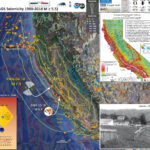
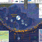
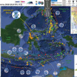
Today I awoke to the USGS earthquake notification service email about an earthquake offshore of Sulawesi, Indonesia. There was an earthquake with a magnitude M 6.8 to the southeast of the Donggala/Palu earthquake from 28 September 2018. Here is the comprehensive earthquake report for the Donggala/Palu earthquake, landslides, and tsunami.
https://earthquake.usgs.gov/earthquakes/eventpage/us700034xq/executive
Just like the September quake, today’s event was a strike-slip earthquake, where the crust moves side-by-side (like the San Andreas fault).
This region of the world is complicated and special. There are subduction zone and transform plate boundaries. I use several maps below to present how these plate boundaries control the types of earthquakes. First I plot the earthquakes from the past year, then for the past century. Of course, let’s remember that seismometers are not that old, so the first half of the 20th century, there were not many seismometers. So, the earthquake record before the 1950s is generally composed of earthquakes with larger magnitude.
There are many many faults in this region, overlapping each other, offsetting each other. And, there have been earthquakes along many of these systems over the past year and past century that represent these different systems and how they interact.

The M 6.8 temblor is strange because it is oriented in a way that is different from the mapped faults in the region. The mainshock/aftershock sequence suggests a northeast-southwest oriented fault (making this a right-lateral strike slip earthquake). The mapped faults with this orientation are instead left-lateral faults.

Below is my interpretive poster for this earthquake

I plot the seismicity from the past month, with color representing depth and diameter representing magnitude (see legend). I include earthquake epicenters from 1918-2018 with magnitudes M ≥ 4.5 and M ≥ 7.5 in different versions.
I plot the USGS fault plane solutions (moment tensors in blue and focal mechanisms in orange), possibly in addition to some relevant historic earthquakes.

  • I placed a moment tensor / focal mechanism legend on the poster. There is more material from the USGS web sites about moment tensors and focal mechanisms (the beach ball symbols). Both moment tensors and focal mechanisms are solutions to seismologic data that reveal two possible interpretations for fault orientation and sense of motion. One must use other information, like the regional tectonics, to interpret which of the two possibilities is more likely.
  • I also include the shaking intensity contours on the map. These use the Modified Mercalli Intensity Scale (MMI; see the legend on the map). This is based upon a computer model estimate of ground motions, different from the “Did You Feel It?” estimate of ground motions that is actually based on real observations. The MMI is a qualitative measure of shaking intensity. More on the MMI scale can be found here and here. This is based upon a computer model estimate of ground motions, different from the “Did You Feel It?” estimate of ground motions that is actually based on real observations.
  • I include the slab 2.0 contours plotted (Hayes, 2018), which are contours that represent the depth to the subduction zone fault. These are mostly based upon seismicity. The depths of the earthquakes have considerable error and do not all occur along the subduction zone faults, so these slab contours are simply the best estimate for the location of the fault.

    Magnetic Anomalies

  • In the M 7.5 map below, I include a transparent overlay of the magnetic anomaly data from EMAG2 (Meyer et al., 2017). As oceanic crust is formed, it inherits the magnetic field at the time. At different points through time, the magnetic polarity (north vs. south) flips, the North Pole becomes the South Pole. These changes in polarity can be seen when measuring the magnetic field above oceanic plates. This is one of the fundamental evidences for plate spreading at oceanic spreading ridges (like the Gorda rise).
  • Regions with magnetic fields aligned like today’s magnetic polarity are colored red in the EMAG2 data, while reversed polarity regions are colored blue. Regions of intermediate magnetic field are colored light purple.
  • We can see the roughly east-west trends of these red and blue stripes. These lines are parallel to the ocean spreading ridges from where they were formed.

    I include some inset figures. Some of the same figures are located in different places on the larger scale map below.

  • In the upper right corner is an overview map from Zahirovic et al. (2014) that shows the major plate boundary faults and tectonic plates. I placed a blue star in the general location of yesterday’s M 6.8 temblor.
  • The map in the upper left corner shows one interpretation of these faults as presented by Bellier et al. (2006). The M 6.8 quake happened somewhere in the intersection of the Batui thrust (an extension of the Molucca Collision) and the Sorong fault. There are half a dozen different interpretations for the tectonics here, this is but one.
  • The map in the lower left corner is a map from Cipta et a. (2006) that shows the relative seismic hazard for Sulawesi. Compare this map with the Bellier map above. Note how the seismic hazard is directly related to the known earthquake faults.
  • In the lower right corner is a low-angle oblique view of the plates and their boundaries in this part of the world (Hall, 2011). I present this figure alone below to highlight the details of how these faults interact near the M 6.8 quake.
  • Here is the map with a year’s seismicity plotted for quakes M ≥ 4.5.
    • Earthquakes from the past year represent well many of the plate boundaries here. Notably is the Donggala/Palu sequence, with all the aftershocks, that align with the trend of the Palu-Koro fault as it connects to the south tot he Sorong fault system.
    • There are several quakes along the Java trench (the Sunda subduction zone), showing thrust quakes (e.g. 2.18, 8.28, and 10.1 in 2018 and 1.21 and 1.22 in 2019). The Lombok sequence of 2018 is also evidence of this north-south convergence.
    • As the Australia plate dives deep beneath the Sunda plate, the slab (the oceanic crust) pulls downwards, causing extension. The 2018.07.28 M 6.0 and 2019.04.06 normal fault earthquakes (orange arrows) are great examples of this. Intermediate depth earthquakes are not completely understood, but we learn more every year. For example, sometimes there are compressional quakes (thrust/reverse) that happen at these depths, e.g. the 2018.08.17 M 6.5 quake.
    • One of the more active regions is the Molucca Strait, where there are subduction/convergent zones that oppose each other. The 2019.01.06 M 6.6 shaker is a good example of what can happen here (and does rather frequently).
    • Further north is the subduction zone that forms the Philippine trench. There was a M 7.0 earthquake on 2018.12.29 that shows evidence of the subduction zone megathrust.


  • Here is the map with a century’s seismicity plotted for quakes M ≥ 7.5.
    • The USGS earthquake catalog includes additional examples of larger quakes over the past century that represent the range of plate boundary types in the region. The global earthquake catalog is better after 1950 due to the increase in seismic monitoring during the cold war (monitoring for nuclear weapons testing).
    • Evidence for subduction along the Sunda subduction zone include subduction zone earthquakes (1977.08.19 M 8.3, 1994.06.02 M 7.8). Also, evidence for down-dip slab-pull extension as evidenced by the 1996.06.17 M 7.9 temblor. similar to the 2018 Lombok sequence, there are also examples of the backthrust to the subduction zone (e.g. 1992.12.12 M 7.8 and 2004.11.11 M 7.5).
    • The Molucca Strait thrust earthquakes are evidence for this bivergent convergence (e.g. 1986.08.14 M 7.5 and 2007.01.21 M 7.5).
    • There is also a subduction zone on the north side of Sulawesi, with several good example earthquakes (e.g. 1990.04.18 M 7.5, 1991.06.20 M 7.5, and 1996.01.01 M 7.9, which was tsunamigenic).
    • There was a strike-slip earthquake on 1998.11.29 that is related to the Sorong fault system, a magnitude M 7.7 shaker.


Other Report Pages

Some Relevant Discussion and Figures

  • This is the small scale tectonic map of the region (Zahirovic et al., 2014). This gives us the overview we need so we can understand the wide variety of plate boundary faults and how they interact with each other.

  • Regional tectonic setting with plate boundaries (MORs/transforms = black, subduction zones = teethed red) from Bird (2003) and ophiolite belts representing sutures modified from Hutchison (1975) and Baldwin et al. (2012). West Sulawesi basalts are from Polvé et al. (1997), fracture zones are from Matthews et al. (2011) and basin outlines are from Hearn et al. (2003). ANI – Andaman and Nicobar Islands, BD– Billiton Depression, Ba – Bangka Island, BI – Belitung (Billiton) Island, BiS – Bismarck Sea, BP – Benham Plateau, CaR – Caroline Ridge, CS – Celebes Sea, DG– Dangerous Grounds, EauR – Eauripik Ridge, FIN – Finisterre Terrane, GoT – Gulf of Thailand, GR– Gagua Ridge, HAL– Halmahera, HBa – Huatung Basin, KB–Ketungau Basin, KP – Khorat Platform, KT – Kiilsgaard Trough, LS – Luconia Shoals, MacB – Macclesfield Bank, ManTr – Manus Trench, MaTr – Mariana Trench, MB– Melawi Basin, MDB– Minami Daito Basin, MG– Mangkalihat, MIN – Mindoro, MN– Mawgyi Nappe, MoS – Molucca Sea, MS– Makassar Straits, MTr – Mussau Trench, NGTr – New Guinea Trench, NI – Natuna Islands, ODR– Oki Daito Ridge, OJP –Ontong Java Plateau, OSF – Owen Stanley Fault, PAL – Palawan, PhF – Philippine Fault, PT – Paternoster Platform, PTr – Palau Trench, PVB – Parece Vela Basin, RB – Reed Bank, RMF– Ramu-Markham Fault, RRF – Red River fault, SEM– Semitau, ShB – Shikoku Basin, Sol. Sea – Solomon Sea, SPK – Sepik, SPT – abah–Palawan Trough, STr – Sorol Trough, Sul – Sulawesi, SuS – Sulu Sea, TPAA– Torricelli–Prince Alexander Arc, WB–West Burma, WCT–W Caroline Trough, YTr –Yap Trough.

  • Here is the tectonic map from Bellier et al., 2006. I include their caption below in blockquote. Note how the Molluca Collision faults trend towards the Batui thrust. However, when we look more closely at the faulting on a local scale, things get much more complicated.


  • Regional geodynamic sketch that presents the present day deformation model of Sulawesi area (after Beaudouin et al., 2003) and four main deformation systems around the Central Sulawesi block, highlighting the tectonic complexity of Sulawesi. Approximate location of the Central Sulawesi block rotation pole (P) [compatible with both GPS measurements (Walpersdorf et al., 1998a) and earthquake moment tensor analyses (Beaudouin et al., 2003)], as well as the major active structures are reported. Central Sulawesi Fault System (CSFS) is formed by the Palu–Koro and Matano faults. Arrows correspond to the compression and/or extension directions deduced from both inversion and moment tensor analyses of the focal mechanisms; arrow size being proportional to the deformation rate (e.g., Beaudouin et al., 2003).We also represent the focal mechanism provided by the Harvard CMT database [CMT data base, 2005] for the recent large earthquake (Mw=6.2; 2005/1/23; lat.=0.928S; long.=120.108E). The box indicates the approximate location of the Fig. 6 that corresponds to the geological map of the Palu basin region. The bottom inset shows the SE Asia and Sulawesi geodynamic frame where arrows represent the approximate Indo-Australian and Philippines plate motions relative to Eurasia.

  • Here is the larger scale map showing the fault configuration in this region (Bellier et al., 2006). I include this so we can see how the Sorong fault system extends and relates to the Palu-Koro system.


  • Sketch map of the Cenozoic Central Sulawesi fault system. ML represents the Matano Lake, and Leboni RFZ, the Leboni releasing fault zone that connects the Palu–Koro and Matano Faults. Triangles indicate faults with reverse component (triangles on the upthrown block). On this map are reported the fault kinematic measurement sites (geographic coordinates in Table 3).

  • Here is the low-angle oblique view of this region. Note the left-lateral strike-slip fault bisecting Sulawesi. Note the Sorong fault system that trends towards this system. The Sorong fault ends in a convergent plate boundary in eastern Sulawesi (the Batui thrust). There is a small north-south fault linking these two systems on the western part of hte N Banda Sea. The M 6.8 earquake happened in this area. We will look at more detailed maps of this area.

  • 3D cartoon of plate boundaries in the Molucca Sea region modified from Hall et al. (1995). Although seismicity identifies a number of plates there are no continuous boundaries, and the Cotobato, North Sulawesi and Philippine Trenches are all intraplate features. The apparent distinction between different crust types, such as Australian continental crust and oceanic crust of the Philippine and Molucca Sea, is partly a boundary inactive since the Early Miocene (east Sulawesi) and partly a younger but now probably inactive boundary of the Sorong Fault. The upper crust of this entire region is deforming in a much more continuous way than suggested by this cartoon.

  • Here is another interpretation showing how these faults map interact in the region (Simandjuntak and Barber, 1996). Yesterday’s M 6.8 quake happened southwest of Banggai.

  • Talaud orogeny in the North Moluccas. Line of section illustrated in Fig. 9 is indicated.

  • This is larger scale, showing details for the Sulawesi region (Simandjuntak and Barber, 1996).

  • Sulawesi orogeny. Line of section illustrated in Fig. 9 is indicated.

  • Below are a couple maps from Watkinson et al. (2011) that show detailed mapping in this area.
  • First here is a fault tectonic map based on new (2011) interpretations. These interpretations are based on detailed seismic reflection data, as well as high resolution multibeam mapping (detailed information about the surface of the seafloor).

  • Map of the same area as Figure 1, and drawn largely after the same sources, but modified in the light of the present study. Revised faults are shown in red. Principal differences include the absence of a through-going Sula Thrust, the Sorong Fault as a plate boundary which does not reach the surface, and connection of the Poh Head fault to the region of dextral transpression in the west of the study area. Sources of deformation in the region are indicated by regions of colour.

  • Here is a regional map showing multibeam bathymetry along with fault line interpretations. This is “figure 3; note the extent for “figure 8,” which is the figure i present next.

  • (a) Shaded relief map of the multibeam data. See inset map for location. Illumination from the NW. (b) Interpreted structural map, showing fault kinematics, basin areas, and fields of debris derived from the collapsing slope in the south. Locations of subsequent figures shown.

  • Here is the detailed map of the seafloor geomorphology (Watkinson et al., 2011). This map is northeast of the island of Banggai, but it informs us about the northeast oriented faults, along with the northwest oriented faults. Note that the northwest oriented faults are right lateral (opposite sense of motion compared to the Sorong fault system, which makes interpreting the M 6.8 more complicated). Also, north how the northwest striking (oriented) faults are left-lateral strike-slip systems. This is also opposite the sense of motion for the M 6.8 earthquake (and also for the 1999.08.12 M 6.2 quake (see the year’s seismicity interpretive poster above).
  • So, we have a mystery. What fault system is responsible for the 2019.04.12 M 6.8 and 1999.08.12 M 6.2 quakes. So exciting!

  • Multibeam image showing details of the region of dextral transpression in the west of the study area. See Figure 3b and inset map for location. Antiformal hinge lines marked by black dashed lines, thrusts marked by white dashed lines. Strike-slip faults marked by double half arrows. Maximum horizontal stress orientations for various structures shown in top right.

  • Next, lets look at the evidence for subduction along the Sunda subduction zone. Below is a map showing historic seismicity (Jones et al., 2014). Cross sections B-B’ and C-C’ are shown. The seismicity for the cross sections below are sourced from within each respective rectangle.

  • Here are the seismcity cross sections.

  • Below are the maps and cross sections from Darman et al., 2012.

  • Tectonic map of the Lesser Sunda Islands, showing the main tectonic units, main faults, bathymetry and location of seismic sections discussed in this paper.

  • Here is the seismicity cross section in the interpretive poster above.

  • This plot shows the earthquake localizations on a South-North cross section for the lat -14°/-4° long 114°/124° quadrant corresponding to the Lesser Sunda Islands region. The localizations are extracted from the USGS database and corresponds to magnitude greater than 4.5 in the 1973-2004 time period (shallow earthquakes with undetermined depth have been omitted.

  • Here is their interpretations of seismic data used to interpret the tectonics of the subduction zone and Flores thrust.

  • Six 15 km deep seismic sections acquired by BGR from west to east traversing oceanic crust, deep sea trench, accretionary prism, outer arc high and fore-arc basin, derived from Kirchoff prestack depth migration (PreSDM) with a frequency range of 4-60 Hz. Profile BGR06-313 shows exemplarily a velocity-depth model according to refraction/wide-angle
    seismic tomography on coincident profile P31 (modified after Lüschen et al, 2011).

Geologic Fundamentals

  • For more on the graphical representation of moment tensors and focal mechanisms, check this IRIS video out:
  • Here is a fantastic infographic from Frisch et al. (2011). This figure shows some examples of earthquakes in different plate tectonic settings, and what their fault plane solutions are. There is a cross section showing these focal mechanisms for a thrust or reverse earthquake. The upper right corner includes my favorite figure of all time. This shows the first motion (up or down) for each of the four quadrants. This figure also shows how the amplitude of the seismic waves are greatest (generally) in the middle of the quadrant and decrease to zero at the nodal planes (the boundary of each quadrant).

  • Here is another way to look at these beach balls.
  • There are three types of earthquakes, strike-slip, compressional (reverse or thrust, depending upon the dip of the fault), and extensional (normal). Here is are some animations of these three types of earthquake faults. The following three animations are from IRIS.
  • Strike Slip:

    Compressional:

    Extensional:

  • This is an image from the USGS that shows how, when an oceanic plate moves over a hotspot, the volcanoes formed over the hotspot form a series of volcanoes that increase in age in the direction of plate motion. The presumption is that the hotspot is stable and stays in one location. Torsvik et al. (2017) use various methods to evaluate why this is a false presumption for the Hawaii Hotspot.

  • A cutaway view along the Hawaiian island chain showing the inferred mantle plume that has fed the Hawaiian hot spot on the overriding Pacific Plate. The geologic ages of the oldest volcano on each island (Ma = millions of years ago) are progressively older to the northwest, consistent with the hot spot model for the origin of the Hawaiian Ridge-Emperor Seamount Chain. (Modified from image of Joel E. Robinson, USGS, in “This Dynamic Planet” map of Simkin and others, 2006.)

  • Here is a map from Torsvik et al. (2017) that shows the age of volcanic rocks at different locations along the Hawaii-Emperor Seamount Chain.

  • Hawaiian-Emperor Chain. White dots are the locations of radiometrically dated seamounts, atolls and islands, based on compilations of Doubrovine et al. and O’Connor et al. Features encircled with larger white circles are discussed in the text and Fig. 2. Marine gravity anomaly map is from Sandwell and Smith.

  • Here is a great tweet that discusses the different parts of a seismogram and how the internal structures of the Earth help control seismic waves as they propagate in the Earth.

    Social Media

    References:

  • Audley-Charles, M.G., 1986. Rates of Neogene and Quaternary tectonic movements in the Southern Banda Arc based on micropalaeontology in: Journal of fhe Geological Society, London, Vol. 143, 1986, pp. 161-175.
  • Audley-Charles, M.G., 2011. Tectonic post-collision processes in Timor, Hall, R., Cottam, M. A. &Wilson, M. E. J. (eds) The SE Asian Gateway: History and Tectonics of the Australia–Asia Collision. Geological Society, London, Special Publications, 355, 241–266.
  • Baldwin, S.L., Fitzgerald, P.G., and Webb, L.E., 2012. Tectonics of the New Guinea Region in Annu. Rev. Earth Planet. Sci., v. 41, p. 485-520.
  • Bellier, O., Se´brier, M., Seward, D., Beaudouin, T., Villeneuve, M., and Putranto, E., 2006. Fission track and fault kinematics analyses for new insight into the Late Cenozoic tectonic regime changes in West-Central Sulawesi (Indonesia) in Tectonophysics, v. 413, p. 201-220.
  • Benz, H.M., Herman, Matthew, Tarr, A.C., Hayes, G.P., Furlong, K.P., Villaseñor, Antonio, Dart, R.L., and Rhea, Susan, 2011. Seismicity of the Earth 1900–2010 New Guinea and vicinity: U.S. Geological Survey Open-File Report 2010–1083-H, scale 1:8,000,000.
  • Cipta, A., Robiana, R., Griffin, J.D., Horspool, N., Hidayati, S., and Cummins, P., 2016. A probabilistic seismic hazard assessment for Sulawesi, Indonesia in Cummins, P. R. &Meilano, I. (eds) Geohazards in Indonesia: Earth Science for Disaster Risk Reduction, Geological Society, London, Special Publications, v. 441, http://doi.org/10.1144/SP441.6
  • Darman, H., 2012. Seismic Expression of Tectonic Features in the Lesser Sunda Islands, Indonesia in Berita Sedimentologi, Indonesian Journal of Sedimentary Geology, no. 25, po. 16-25.
  • Frisch, W., Meschede, M., Blakey, R., 2011. Plate Tectonics, Springer-Verlag, London, 213 pp.
  • Gómez, J.M., Madariaga, R., Walpersdorf, A., and Chalard, E., 2000. The 1996 Earthquakes in Sulawesi, Indonesia in BSSA, v. 90, no. 3, p. 739-751
  • Hall, R., 2011. Australia-SE Asia collision: plate tectonics and crustal flow in Geological Society, London, Special Publications 2011; v. 355; p. 75-109 doi: 10.1144/SP355.5
  • Hangesh, J. and Whitney, B., 2014. Quaternary Reactivation of Australia’s Western Passive Margin: Inception of a New Plate Boundary? in: 5th International INQUA Meeting on Paleoseismology, Active Tectonics and Archeoseismology (PATA), 21-27 September 2014, Busan, Korea, 4 pp.
  • Hayes, G., 2018, Slab2 – A Comprehensive Subduction Zone Geometry Model: U.S. Geological Survey data release, https://doi.org/10.5066/F7PV6JNV.
  • Jones, E.S., Hayes, G.P., Bernardino, Melissa, Dannemann, F.K., Furlong, K.P., Benz, H.M., and Villaseñor, Antonio, 2014. Seismicity of the Earth 1900–2012 Java and vicinity: U.S. Geological Survey Open-File Report 2010–1083-N, 1 sheet, scale 1:5,000,000, https://dx.doi.org/10.3133/ofr20101083N.
  • Koulali, A., S. Susilo, S. McClusky, I. Meilano, P. Cummins, P. Tregoning, G. Lister, J. Efendi, and M. A. Syafi’i, 2016. Crustal strain partitioning and the associated earthquake hazard in the eastern Sunda-Banda Arc in Geophys. Res. Lett., 43, 1943–1949, doi:10.1002/2016GL067941
  • Lin, J., and R. S. Stein (2004), Stress triggering in thrust and subduction earthquakes and stress interaction between the southern San Andreas and nearby thrust and strike-slip faults, J. Geophys. Res., 109, B02303, doi:10.1029/2003JB002607.
  • Lüschen, E., Müller, C., Kopp, H., Engels, M., Lutz, R., Planert, L., Shulgin, A., Djajadihardja, Y. S., 2011. Structure, evolution and tectonic activity of the eastern Sunda forearc,Indonesia from marine seismic investigations, Tectonophysics, 508, p. 6-21
  • McCaffrey, R., and Nabelek, J.L., 1984. The geometry of back arc thrusting along the Eastern Sunda Arc, Indonesia: Constraints from earthquake and gravity data in JGR, Atm., vol., 925, no. B1, p. 441-4620, DOI: 10.1029/JB089iB07p06171
  • Meyer, B., Saltus, R., Chulliat, a., 2017. EMAG2: Earth Magnetic Anomaly Grid (2-arc-minute resolution) Version 3. National Centers for Environmental Information, NOAA. Model. https://doi.org/10.7289/V5H70CVX
  • Müller, R.D., Sdrolias, M., Gaina, C. and Roest, W.R., 2008, Age spreading rates and spreading asymmetry of the world’s ocean crust in Geochemistry, Geophysics, Geosystems, 9, Q04006, https://doi.org/10.1029/2007GC001743
  • Okal, E. A., & Reymond, D., 2003. The mechanism of great Banda Sea earthquake of 1 February 1938: applying the method of preliminary determination of focal mechanism to a historical event in EPSL, v. 216, p. 1-15.
  • Silver, E.A., Breen, N.A., and Prastyo, H., 1986. Multibeam Study of the Flores Backarc Thrust Belt, Indonesia, in JGR., vol. 91, no. B3, p. 3489-3500
  • Simandjuntak, T.O. and Barber, A.J., 1996. Contrasting tectonic styles in the Neogene orogenic belts of Indonesia in Hall, R. & Blundell, D. (eds), 1996, Tectonic Evolution of Southeast Asia, Geological Society Special Publication No. 106, pp. 185-201.
  • Socquet, A., Simons, W., Vigny, C., McCaffrey, R., Subarya, C., Sarsito, D., Ambrosius, B., and Spakman, W., 2006. Microblock rotations and fault coupling in SE Asia triple junction (Sulawesi, Indonesia) from GPS and earthquake slip vector data, J. Geophys. Res., 111, B08409, doi:10.1029/2005JB003963.
  • Walpersdorf, A., Rangin, C., and Vigny, C., 1998. GPS compared to long-term geologic motion of the north arm of Sulawesi in EPSL, v. 159, p. 47-55.
  • Watkinson, I.M. Hall, R., Ferdian, F., 2011. Tectonic re-interpretation of the Banggai-Sula–Molucca Sea margin, Indonesia in Hall, R., Cottam, M. A. &Wilson, M. E. J. (eds) The SE Asian Gateway: History and Tectonics of the Australia–Asia Collision. Geological Society, London, Special Publications, 355, 203–224. http://doi.org/10.1144/SP355.10
  • Watkinson, I.M. and Hall, R., 2017. Fault systems of the eastern Indonesian triple junction: evaluation of Quaternary activity and implications for seismic hazards in Cummins, P. R. & Meilano, I. (eds) Geohazards in Indonesia: Earth Science for Disaster Risk Reduction, Geological Society, London, Special Publications, v. 441, https://doi.org/10.1144/SP441.8
  • Zahirovic, S., Seton, M., and Müller, R.D., 2014. The Cretaceous and Cenozoic tectonic evolution of Southeast Asia in Solid Earth, v. 5, p. 227-273, doi:10.5194/se-5-227-2014

Return to the Earthquake Reports page.


18 April 1906 San Francisco Earthquake

Today is the anniversary of the 18 April 1906 San Francisco Earthquake. There are few direct observations (e.g. from seismometers or other instruments) from this earthquake, so our knowledge of how strong the ground shook during the earthquake are limited to indirect measurements.
Below I present a poster that shows a computer simulation that provides an estimate of the intensity of the ground shaking that may happen if the San Andreas fault slipped in a similar way that it did in 1906.
The USGS prepares these ShakeMap scenario maps so that we can have an estimate of the ground shaking from hypothetical earthquakes. I present a poster below that uses data from one of these scenarios. This is a scenario that is similar to what we think happened in 1906, but it is only a model.
There is lots about the 1906 Earthquake that I did not include, but this leaves me room for improvement for the years into the future, when we see this anniversary come again.

Below is my interpretive poster for this earthquake

I plot the seismicity from the past month, with color representing depth and diameter representing magnitude (see legend). I include earthquake epicenters from 1900-2018 with magnitudes M ≥ 5.5.
I plot the USGS fault plane solutions (moment tensors in blue and focal mechanisms in orange), possibly in addition to some relevant historic earthquakes.

  • I placed a moment tensor / focal mechanism legend on the poster. There is more material from the USGS web sites about moment tensors and focal mechanisms (the beach ball symbols). Both moment tensors and focal mechanisms are solutions to seismologic data that reveal two possible interpretations for fault orientation and sense of motion. One must use other information, like the regional tectonics, to interpret which of the two possibilities is more likely.
  • I also include the shaking intensity contours on the map. These use the Modified Mercalli Intensity Scale (MMI; see the legend on the map). This is based upon a computer model estimate of ground motions, different from the “Did You Feel It?” estimate of ground motions that is actually based on real observations. The MMI is a qualitative measure of shaking intensity. More on the MMI scale can be found here and here. This is based upon a computer model estimate of ground motions, different from the “Did You Feel It?” estimate of ground motions that is actually based on real observations.

    Magnetic Anomalies

  • In the map below, I include a transparent overlay of the magnetic anomaly data from EMAG2 (Meyer et al., 2017). As oceanic crust is formed, it inherits the magnetic field at the time. At different points through time, the magnetic polarity (north vs. south) flips, the North Pole becomes the South Pole. These changes in polarity can be seen when measuring the magnetic field above oceanic plates. This is one of the fundamental evidences for plate spreading at oceanic spreading ridges (like the Gorda rise).
  • Regions with magnetic fields aligned like today’s magnetic polarity are colored red in the EMAG2 data, while reversed polarity regions are colored blue. Regions of intermediate magnetic field are colored light purple.
  • We can see the roughly north-south trends of these red and blue stripes. These lines are parallel to the ocean spreading ridges from where they were formed.

    I include some inset figures. Some of the same figures are located in different places on the larger scale map below.

  • On the right is a map from Wallace (1990) that shows the main faults that are part of the Pacific – North America plate boundary. The San Andreas fault is the locus of a majority of this relative plate motion.
  • In the upper right, to the left of the Wallace map, is a map of the entire state of California. This map shows the shaking potential for different regions based on an estimate of earthquake probability. Pink areas are more likely to experience stronger ground shaking, more frequently, than areas colored green.
  • In the lower right, to the left of the Wallace map, is a photo showing a fence that was offset during the 1906 earthquake. The relative distance between these fences is about 2.6 meters (Lawson, 1908; Aargard and Bowza, 2008).
  • In the upper left corner is a map showing an estimate of the ground motions produced by the 1906 San Francisco earthquake, based on Song et al. (2008) source model (Aargard et al., 2008).
  • In the lower left corner is a figure that shows the historic earthquakes for hte San Francisco Bay region (Aagaard et al., 2016). Note that they find there to be a 72% chance of an earthquake with manitude 6.7 or greater between 2014 and 2043.
  • Here is the map with a month’s seismicity plotted.

  • Here is the photo of the offset fence (Aargard and Bowza, 2008).

  • Fence half a mile northwest of Woodville (east of Point Reyes), offset by approximately 2.6 m of right-lateral strike-slip motion on the San Andreas fault in the 1906 San Francisco earthquake (U.S. Geological Survey Photographic Library, Gilbert, G. K. 2845).

  • Here is the USGS ShakeMap (Aargard et al., 2008)

  • ShakeMap for the 1906 San Francisco earthquake based on the Boatwright and Bundock (2005) intensities (processed 18 October 2005). Open circles identify the intensity sites used to construct the ShakeMap.

  • In the map above, we can see that the ground shaking was quite high in Humboldt County, CA. Below is a photo from Dengler et al. (2008) that shows headscarps to some lateral slides that failed as a result of the 1906 earthquake. This is the tupe of failure that extended across a much larger landscape for the 28 September 2018 Dongalla / Palu earthquake and tsunami.

  • Spread failures on the banks of the Eel River near Port Kenyon in 1906. Photo E. Garrett, courtesy of Peter Palmquist.

  • Here is a map that shows the estimate for the location of the epicenter for the mainshock of the 1906 earthquake. See Lomax (2008) for more on this.

  • I place a map shows the configuration of faults in central (San Francisco) and northern (Point Delgada – Punta Gorda) CA (Wallace, 1990). Here is the caption for this map, that is on the lower left corner of my map. Below the citation is this map presented on its own.

  • Geologic sketch map of the northern Coast Ranges, central California, showing faults with Quaternary activity and basin deposits in northern section of the San Andreas fault system. Fault patterns are generalized, and only major faults are shown. Several Quaternary basins are fault bounded and aligned parallel to strike-slip faults, a relation most apparent along the Hayward-Rodgers Creek-Maacama fault trend.

  • Here is the figure showing the evolution of the SAF since its inception about 29 Ma. I include the USGS figure caption below as a blockquote.

  • EVOLUTION OF THE SAN ANDREAS FAULT.
    This series of block diagrams shows how the subduction zone along the west coast of North America transformed into the San Andreas Fault from 30 million years ago to the present. Starting at 30 million years ago, the westward- moving North American Plate began to override the spreading ridge between the Farallon Plate and the Pacific Plate. This action divided the Farallon Plate into two smaller plates, the northern Juan de Fuca Plate (JdFP) and the southern Cocos Plate (CP). By 20 million years ago, two triple junctions began to migrate north and south along the western margin of the West Coast. (Triple junctions are intersections between three tectonic plates; shown as red triangles in the diagrams.) The change in plate configuration as the North American Plate began to encounter the Pacific Plate resulted in the formation of the San Andreas Fault. The northern Mendicino Triple Junction (M) migrated through the San Francisco Bay region roughly 12 to 5 million years ago and is presently located off the coast of northern California, roughly midway between San Francisco (SF) and Seattle (S). The Mendicino Triple Junction represents the intersection of the North American, Pacific, and Juan de Fuca Plates. The southern Rivera Triple Junction (R) is presently located in the Pacific Ocean between Baja California (BC) and Manzanillo, Mexico (MZ). Evidence of the migration of the Mendicino Triple Junction northward through the San Francisco Bay region is preserved as a series of volcanic centers that grow progressively younger toward the north. Volcanic rocks in the Hollister region are roughly 12 million years old whereas the volcanic rocks in the Sonoma-Clear Lake region north of San Francisco Bay range from only few million to as little as 10,000 years old. Both of these volcanic areas and older volcanic rocks in the region are offset by the modern regional fault system. (Image modified after original illustration by Irwin, 1990 and Stoffer, 2006.)

Tectonic History of Western North America and Southern California

  • Here is an animation from Tanya Atwater that shows how the Pacific-North America plate margin evolved over the past 40 million years (Ma).

Some Relevant Discussion and Figures

  • Here is the shaking potential map for California.

  • Here is the earthquake timeline (Aagaard et al., 2016).

  • This map shows the relative contribution that each fault has for the chance of earthquakes in the region. For example, this shows that the Hayward fault is the fault with the highest chance of rupture (Aagaard et al., 2016).

Geologic Fundamentals

  • For more on the graphical representation of moment tensors and focal mechanisms, check this IRIS video out:
  • Here is a fantastic infographic from Frisch et al. (2011). This figure shows some examples of earthquakes in different plate tectonic settings, and what their fault plane solutions are. There is a cross section showing these focal mechanisms for a thrust or reverse earthquake. The upper right corner includes my favorite figure of all time. This shows the first motion (up or down) for each of the four quadrants. This figure also shows how the amplitude of the seismic waves are greatest (generally) in the middle of the quadrant and decrease to zero at the nodal planes (the boundary of each quadrant).

  • Here is another way to look at these beach balls.
  • There are three types of earthquakes, strike-slip, compressional (reverse or thrust, depending upon the dip of the fault), and extensional (normal). Here is are some animations of these three types of earthquake faults. The following three animations are from IRIS.
  • Strike Slip:

    Compressional:

    Extensional:

  • This is an image from the USGS that shows how, when an oceanic plate moves over a hotspot, the volcanoes formed over the hotspot form a series of volcanoes that increase in age in the direction of plate motion. The presumption is that the hotspot is stable and stays in one location. Torsvik et al. (2017) use various methods to evaluate why this is a false presumption for the Hawaii Hotspot.

  • A cutaway view along the Hawaiian island chain showing the inferred mantle plume that has fed the Hawaiian hot spot on the overriding Pacific Plate. The geologic ages of the oldest volcano on each island (Ma = millions of years ago) are progressively older to the northwest, consistent with the hot spot model for the origin of the Hawaiian Ridge-Emperor Seamount Chain. (Modified from image of Joel E. Robinson, USGS, in “This Dynamic Planet” map of Simkin and others, 2006.)

  • Here is a map from Torsvik et al. (2017) that shows the age of volcanic rocks at different locations along the Hawaii-Emperor Seamount Chain.

  • Hawaiian-Emperor Chain. White dots are the locations of radiometrically dated seamounts, atolls and islands, based on compilations of Doubrovine et al. and O’Connor et al. Features encircled with larger white circles are discussed in the text and Fig. 2. Marine gravity anomaly map is from Sandwell and Smith.

  • Here is a great tweet that discusses the different parts of a seismogram and how the internal structures of the Earth help control seismic waves as they propagate in the Earth.

    Social Media

Return to the Earthquake Reports page.


Earthquake Report: central Aleutians

A couple days ago, in my inbox, there was an email from the Pacific Tsunami Warning Center about an earthquake along the Aleutian Islands, near Rat Island, Alaska. However, this earthquake was not along the megathrust subduction zone fault there and it was rather deep (~19 km). Also, this earthquake was strike-slip (not thrust or reverse), so probably did not produce much vertical ground motion. These two factors combined (deep and strike-slip) suggest to me that there would not be a tsunami generated from this earthquake. BUT we learn new things every month.
https://earthquake.usgs.gov/earthquakes/eventpage/us2000k9d7/executive
There was a subduction zone earthquake nearby on 15 August 2018. Learn more about the subduction zone in my earthquake report for this M 6.6 earthquake here.
There was a similar earthquake in 2017 further to the west, which was also a strike-slip earthquake and it produced a small sized tsunami (Lay et al., 2017). However, the 17 July 2017 magnitude M 7.9 earthquake was much larger in magnitude. Here is my earthquake report and update for this 2017 earthquake. These reports include information about the intersection of the Aleutian and Kuril plate boundaries.
The majority of the Aleutian Islands are volcanic arc islands formed as a result of the subduction of the Pacific plate beneath the North America plate. To the west, there is another subduction zone along the Kuril and Kamchatka volcanic arcs. These subduction zones form deep sea trenches (the deepest parts of the ocean are in subduction zone trenches).
In the eastern part of the Aleutian/Alaska subduction zone (e.g. Alaska Peninsula or Prince William Sound), the plates converge in the direction of subduction (perpendicular to the fault orientation or “strike”). Further to the west, the plates converge obliquely compared to the fault orientation.
This oblique convergence results in the development of additional special faults that accommodate the plate convergence not perpendicular to the faults. These are typically strike-slip faults parallel to the subduction zone (they accommodate the proportion of relative motion parallel to the fault), called forearc sliver faults.
Along the central and western Aleutian plate boundary, this strike-slip relative motion also creates blocks in the upper North America plate that rotate relative to the forearc sliver fault. Imagine how ball bearings rotate when the two planes that they are contained within move relative to each other.

Below is my interpretive poster for this earthquake

I plot the seismicity from the past month, with color representing depth and diameter representing magnitude (see legend). I include earthquake epicenters from 1918-2018 with magnitudes M ≥ 6.5 in one version.
I plot the USGS fault plane solutions (moment tensors in blue and focal mechanisms in orange), possibly in addition to some relevant historic earthquakes.

  • I placed a moment tensor / focal mechanism legend on the poster. There is more material from the USGS web sites about moment tensors and focal mechanisms (the beach ball symbols). Both moment tensors and focal mechanisms are solutions to seismologic data that reveal two possible interpretations for fault orientation and sense of motion. One must use other information, like the regional tectonics, to interpret which of the two possibilities is more likely.
  • I also include the shaking intensity contours on the map. These use the Modified Mercalli Intensity Scale (MMI; see the legend on the map). This is based upon a computer model estimate of ground motions, different from the “Did You Feel It?” estimate of ground motions that is actually based on real observations. The MMI is a qualitative measure of shaking intensity. More on the MMI scale can be found here and here. This is based upon a computer model estimate of ground motions, different from the “Did You Feel It?” estimate of ground motions that is actually based on real observations.
  • I include the slab 2.0 contours plotted (Hayes, 2018), which are contours that represent the depth to the subduction zone fault. These are mostly based upon seismicity. The depths of the earthquakes have considerable error and do not all occur along the subduction zone faults, so these slab contours are simply the best estimate for the location of the fault.

    Magnetic Anomalies

  • In the map below, I include a transparent overlay of the magnetic anomaly data from EMAG2 (Meyer et al., 2017). As oceanic crust is formed, it inherits the magnetic field at the time. At different points through time, the magnetic polarity (north vs. south) flips, the North Pole becomes the South Pole. These changes in polarity can be seen when measuring the magnetic field above oceanic plates. This is one of the fundamental evidences for plate spreading at oceanic spreading ridges (like the Gorda rise).
  • Regions with magnetic fields aligned like today’s magnetic polarity are colored red in the EMAG2 data, while reversed polarity regions are colored blue. Regions of intermediate magnetic field are colored light purple.
  • We can see the roughly east-west trends of these red and blue stripes. These lines are parallel to the ocean spreading ridges from where they were formed. The stripes disappear at the subduction zone because the oceanic crust with these anomalies is diving deep beneath the North America plate \, so the magnetic anomalies from the overlying North America plate mask the evidence for the Pacific plate.

    I include some inset figures. Some of the same figures are located in different places on the larger scale map below.

  • In the lower right corner is a figure that shows the historic earthquake ruptures along the Aleutian Megathrust (Peter Haeussler, USGS). I placed a blue star in the general location of this M 6.5 quake (same for the other inset figures).
  • In the upper left corner is a figure that shows how oblique relative motion between plates results in a variety of faults and fault bounded blocks (Lange et al., 2008). This example is from southern Chile (near the 1960 subduction zone earthquake).
  • In the upper right corner is a plate tectonic map showing the plate boundaries (inset) and the crustal faults in the North America plate (Krutikov et al., 2008). The wide arrows show motion of Pacific plate relative to the North America plate (the direction the plate is subducting). These authors used the paleomagnetic data as evidence for rotation of fault bounded blocks.
  • In the lower left corner is a figure from Bassett and Watts (2015 B) that shows the results of their analyses using gravity data.
  • Here is the map with a month’s seismicity plotted. I outlined the blocks and labeled using Ryan and Scholl (1989) as a basemap (but very similar to Krutikov). I outlined some lineaments in the magnetic anomaly data for crust on both sides of the Amlia fracture zone and labeled these B and A (near label for Pacific plate). Note how they are offset relative to each other, demonstration of the left-lateral sense of motion here.

  • Here is the map with a century’s seismicity plotted. Check out the example strike slip earthquakes, including the 2017.06.02 M 6.8 quake (that was interpreted by Lay et al., 2017 to be right lateral). Also shown is the 2003.11.17 M 7.8 subduction earthquake. Many of the other earthquakes plotted in this map are also subduction earthquakes.

  • Here is the map with a century’s seismicity plotted, with megathrust earthquake patches from Peter Haeussler (USGS) outlined. I outlined the subduction zone slip patches shown in the Peter Haeussler (USGS) map. Consider how the structures in the different plates may interact with each other.

Other Report Pages

Some Relevant Discussion and Figures

  • Here is a map that shows historic earthquake slip regions as pink polygons (Peter Haeussler, USGS). Dr. Haeussler also plotted the magnetic anomalies (grey regions), the arc volcanoes (black diamonds), and the plate motion vectors (mm/yr, NAP vs PP).

  • Here is the figure from Sykes et al. (1980) that shows the space time relations for historic earthquakes in relation to the map.

  • Above: Rupture zones of earthquakes of magnitude M > 7.4 from 1925-1971 as delineated by their aftershocks along plate boundary in Aleutians, southern Alaska and offshore British Columbia [after Sykes, 1971]. Contours in fathoms. Various symbols denote individual aftershock sequences as follows: crosses, 1949, 1957 and 1964; squares, 1938, 1958 and 1965; open triangles, 1946; solid triangles, 1948; solid circles, 1929, 1972. Larger symbols denote more precise locations. C = Chirikof Island. Below: Space-time diagram showing lengths of rupture zones, magnitudes [Richter, 1958; Kanamori, 1977 b; Kondorskay and Shebalin, 1977; Kanamori and Abe, 1979; Perez and Jacob, 1980] and locations of mainshocks for known events of M > 7.4 from 1784 to 1980. Dashes denote uncertainties in size of rupture zones. Magnitudes pertain to surface wave scale, M unless otherwise indicated. M is ultra-long period magnitude of Kanamori 1977 b; Mt is tsunami magnitude of Abe[ 1979]. Large shocks 1929 and 1965 that involve normal faulting in trench and were not located along plate interface are omitted. Absence of shocks before 1898 along several portions of plate boundary reflects lack of an historic record of earthquakes for those areas.

  • Here is a great illustration that shows how forearc sliver faults form due to oblique convergence at a subduction zone (Lange et al., 2008). Strain is partitioned into fault normal faults (the subduction zone) and fault parallel faults (the forearc sliver faults, which are strike-slip). This figure is for southern Chile, but is applicable globally.

  • Proposed tectonic model for southern Chile. Partitioning of the oblique convergence vector between the Nazca plate and South American plate results in a dextral strike-slip fault zone in the magmatic arc and a northward moving forearc sliver. Modified after Lavenu and Cembrano (1999).

  • Here is a figure from Krutikov et al. (2008) that shows how blocks in the Aleutian Arc may accommodate the oblique subduction, along forearc sliver faults. Note that these blocks may also rotate to accommodate the oblique convergence. There are also margin parallel strike slip faults that bound these blocks. These faults are in the upper plate, but may impart localized strain to the lower plate, resulting in strike slip motion on the lower plate (my arm waving part of this). Note how the upper plate strike-slip faults have the same sense of motion as these deeper earthquakes.

  • Location map for the Aleutian Islands. The outline blocks and shaded summit basins are from Geist et al. [1988], showing a possible rotation mechanism. The heavy arrows show the mean rotations with respect to North America indicated by paleomagnetic data, the lighter arrows the motion of the Pacific plate with respect to North America. (inset) General location map modified from Chapman and Solomon [1976], Mackey et al. [1997], and Pedoja et al. [2006]. Solid lines show boundaries of plates and blocks: NA, North American Plate; B, Bering Block; PA, Pacific Plate; OKH, Okhotsk Plate; KI, Komandorsky Island Block; EUA, Eurasian Plate

  • Here is a figure from Ryan and Scholl (1989) that shows their interpretation of the fault bounded blocks within the forearc shear couple.

  • Map showing the boundaries of clockwise-rotating and westward translating blocks that comprise the Aleutian Ridge [from Geist et al. 1988]. Summit basins and transverse Pacific slope canyons are extensional structures that formed in the wake of these rotating and translating blocks. Arrows show relative plate motion between the Pacific and North American plates; convergence is increasingly oblique to the west. The central Aleutian sector lies within the Andreanof block located between Adak Canyon and Amukta Basin. A prominent summit basin has formed in the eastern part of the block (the composite Amlia and Amukta Basins). However, a summit basin is not present in the western part of the Andreanof block between Adak and Atka Islands. Asterisks show the location of active and dormant volcanoes; the star denotes the approximate location of the 1986 Andreanof earthquake.

  • This is a figure from Lay et al. (2017) that shows their estimate for fault slip for the 2017 temblor. This shows a northwest-southeast trending (striking) strike-slip fault. This is the slip model they used as input for their tsunami model.

  • (a) Bilateral slip model for the 2017 earthquake and USGS/NEIC catalog seismicity from 1900 to 16 July 2017 (blue circles, scaled proportional to magnitude, with events larger than M ~ 7 being labeled), along with all moment tensor solutions from the GCMT catalog from 1976 to 16 July 2017 (red-filled compressional quadrant focal mechanisms). (b) Foreshock seismicity on 17 July 2017 (blue circles) and aftershock seismicity in the first 2 weeks (magenta circles) along with the MW 6.3 foreshock GCMT focal mechanism (cyan focal mechanism). The large focal mechanism is the W-phase moment tensor from this study. The boxes indicate short-period radiators from the Eurasia-Greenland back projection, and stars indicate radiators from the North American back projection (Figure 3). The slip distribution is shown in detail in Figure S12. White vectors indicate the relative motion of the Pacific Plate to North America (almost identical to that relative to the Bering Plate). The large red star indicates the main shock epicenter.

  • Here is a figure from Lay et al. (2017) that shows (a) their initial condition (the amount of seafloor vertical land motion that initiated the tsunami, (b) the maximum wave height map, and (c) the comparison between their model results (in red) and the observations (in black) for water surface elevations after the earthquake.

  • Predicted tsunami from the bilateral faulting model. (a) Final seafloor deformation with the red star indicating the epicenter and the dashed line delineating projection of the faulting model on the seafloor. (b) Predicted tsunami amplitude and DART stations (circles) considered in this study. (c) Comparison of filtered sea surface recordings (black) at DART stations with predictions (red) along with corresponding amplitude spectra (right). The recorded and predicted time series were filtered to remove signals shorter than 5 min period and the full 5 h time series were used in the computation of the amplitude spectra. The strike-slip faulting and position of the stations result in weak tsunami waves, but the timing and height of long-period arrivals provide bounds on the source.

  • Here is the figure from Bassett and Watts (2015) for the Aleutians.

  • Aleutian subduction zone. Symbols as in Figure 3. (a) Residual free-air gravity anomaly and seismicity. The outer-arc high, trench-parallel fore-arc ridge and block-bounding faults are dashed in blue, black, and red, respectively. Annotations are AP = Amchitka Pass; BHR = Black-Hills Ridge; SS = Sunday Sumit Basin; PD = Pratt Depression. (b) Published asperities and slip-distributions/aftershock areas for large magnitude earthquakes. (c) Cross sections showing residual bathymetry (green), residual free-air gravity anomaly (black), and the geometry of the seismogenic zone [Hayes et al., 2012].

  • Here is the schematic figure from Bassett and Watts (2015).

  • Schematic diagram summarizing the key spatial associations interpreted between the morphology of the fore-arc and variations in the seismogenic behavior of subduction megathrusts.

  • Here are several figures from Konstantnovskaia et al. (2001) showing their tectonic reconstructions. I include their figure captions below in blockquote. The first figure is the one included in the poster above.

  • Geodynamic setting of Kamchatka in framework of the Northwest Pacific. Modified after Nokleberg et al. (1994) and Kharakhinov (1996)). Simplified cross-section line I-I’ is shown in Fig. 2. The inset shows location of Sredinny and Eastern Ranges. [More figure caption text in the publication].

  • Here are 4 panels that show the details of their reconstructions. Panels shown are for 65 Ma, 55 Ma, 37 Ma, and Present.


  • The Cenozoic evolution in the Northwest Pacific. Plate kinematics is shown in hotspot reference frame after (Engebretson et al., 1985). Keys distinguish zones of active volcanism (thick black lines), inactive volcanic belts (thick gray lines), deformed arc terranes (hatched pattern), subduction zones: active (black triangles), inactive *(empty triangles). In letters: sa = Sikhote-aline, bs = Bering shelf belts; SH = Shirshov Ridge; V = Vitus arch; KA = Kuril; RA = Ryukyu’ LA = Luzon; IBMA = Izu-Bonin-Mariana arcs; WPB = Western Philippine, BB = Bowers basins.

  • Here is a beautiful illustration for the Aleutian Trench from Alpha (1973) as posted on the David Rumsey Collection online.

Geologic Fundamentals

  • For more on the graphical representation of moment tensors and focal mechanisms, check this IRIS video out:
  • Here is a fantastic infographic from Frisch et al. (2011). This figure shows some examples of earthquakes in different plate tectonic settings, and what their fault plane solutions are. There is a cross section showing these focal mechanisms for a thrust or reverse earthquake. The upper right corner includes my favorite figure of all time. This shows the first motion (up or down) for each of the four quadrants. This figure also shows how the amplitude of the seismic waves are greatest (generally) in the middle of the quadrant and decrease to zero at the nodal planes (the boundary of each quadrant).

  • Here is another way to look at these beach balls.
  • There are three types of earthquakes, strike-slip, compressional (reverse or thrust, depending upon the dip of the fault), and extensional (normal). Here is are some animations of these three types of earthquake faults. The following three animations are from IRIS.
  • Strike Slip:

    Compressional:

    Extensional:

  • This is an image from the USGS that shows how, when an oceanic plate moves over a hotspot, the volcanoes formed over the hotspot form a series of volcanoes that increase in age in the direction of plate motion. The presumption is that the hotspot is stable and stays in one location. Torsvik et al. (2017) use various methods to evaluate why this is a false presumption for the Hawaii Hotspot.

  • A cutaway view along the Hawaiian island chain showing the inferred mantle plume that has fed the Hawaiian hot spot on the overriding Pacific Plate. The geologic ages of the oldest volcano on each island (Ma = millions of years ago) are progressively older to the northwest, consistent with the hot spot model for the origin of the Hawaiian Ridge-Emperor Seamount Chain. (Modified from image of Joel E. Robinson, USGS, in “This Dynamic Planet” map of Simkin and others, 2006.)

  • Here is a map from Torsvik et al. (2017) that shows the age of volcanic rocks at different locations along the Hawaii-Emperor Seamount Chain.

  • Hawaiian-Emperor Chain. White dots are the locations of radiometrically dated seamounts, atolls and islands, based on compilations of Doubrovine et al. and O’Connor et al. Features encircled with larger white circles are discussed in the text and Fig. 2. Marine gravity anomaly map is from Sandwell and Smith.

  • Here is a great tweet that discusses the different parts of a seismogram and how the internal structures of the Earth help control seismic waves as they propagate in the Earth.

    Social Media

Return to the Earthquake Reports page.