Earthquake Report: San Pablo Bay, CA

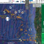
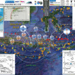
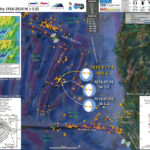
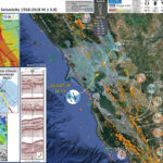
Well well.
There was a small earthquake in the San Francisco Bay area today, with an epicenter in San Pablo Bay northwest of Richmond and San Pablo, CA. This earthquake is cool, at least in part, because of its location.
There are several fault systems that bisect the SF Bay area, which are all part of the San Andreas fault system, the right-lateral strike-slip plate boundary between the North America and Pacific plates. A large proportion of the relative motion along this plate boundary is localized on the San Andreas fault proper. The faults in the SF Bay area are thought to accommodate 85% of the plate boundary relative motion. The rest of this boundary relative motion can be observed along the east side of the Sierra Nevada, with smaller proportions extending through central Nevada and as far east as the Wasatch fault system in Utah.
The San Andreas and sister faults initiated this right-lateral relative motion at the plate boundary approximately 29 million years ago, in a location near where Los Angeles currently is. Over time, various subparallel strike-slip faults have formed. The main strands in the SF Bay area are the San Gregorio, San Andreas, Hayward – Rogers Creek, Maacama, Calaveras – Paicines, and Hunting Creek – Berryessa – Green Valley – Concord – Greenville fault systems. Geologists have been debating about how the Hayward and Rogers Creek faults interact.
The cool part about the location of this earthquake is that it happened in a place that holds great interest to those in the seismic hazard community. In the SF Bay area, the Hayward – Rogers Creek fault system is the fault that has the highest probability of having an earthquake with a magnitude of M 6.7. There is a 33% chance that there will be a M ≥ 6.7 earthquake between 2014 and 2043.
Some have proposed that there is a step over, where these two faults overlap and there is some proportion of extension in this transfer zone. This hypothesis includes the idea that ruptures here may cause subsidence between the fault strands, causing a local tsunami in the area.
Others hypothesize that these faults are more directly linked. USGS geologists like Janet Watt have been conducting seismic reflection and sediment coring studies to evaluate this likelihood. Here is a review of their work in San Pablo Bay.

    From the USGS: Why does it matter?

  • The longer the stretch of fault that breaks during an earthquake, the stronger the quake. When two faults are close to one another, the earthquake can jump from one to the other, making the rupture longer and the shaking stronger. When two faults are directly connected, it’s even easier for earthquake rupture to continue from one fault to the next.
  • A break along the combined length of the Hayward and Rodgers Creek faults could produce a major earthquake of magnitude 7.4. That earthquake would release more than five times the energy released by the 1989 magnitude 6.9 Loma Prieta earthquake, which caused about $6 billion in damage and killed 63 people.
  • To estimate the earthquake hazard posed by the Hayward and Rodgers Creek faults, scientists need to understand whether and how the faults connect. Previous work showed that the two faults approach each other closely beneath San Pablo Bay, but their exact relationship remained a mystery.

The USGS researchers found that the Hayward fault appears to connect directly to the Rodgers Creek fault.

    From the USGS: Unexpected trajectory

  • “Where the faults enter San Pablo Bay, the Hayward from the south and the Rodgers Creek from the north, their orientations suggest that they’ll run parallel to one another, separated by a space, or ‘stepover,’ of about 5 kilometers [3 miles],” said Janet Watt, USGS research geophysicist and lead author of the study. “So when we went out to map, we thought we were going to map details of the stepover—like minor fractures that might enable an earthquake rupture to cross from one fault to the other.”
  • As the data accumulated, however, the researchers saw that the Hayward fault strand they were mapping bends slightly to the right as it traverses San Pablo Bay, heading toward the Rodgers Creek fault.
  • They realized that they might be looking at a fault bend. The distinction is important because fault bends affect earthquake hazards differently than stepovers. These differences include how likely a break on one fault will continue on to the next, how much slip (movement of rock on either side of the fault) will occur, and where ground shaking will be strongest.

Another cool thing about today’s earthquake is that this year marks the anniversary of the last major earthquake on the Hayward fault in 1868. The USGS, CGS, and other organizations and agencies are rolling out Haywired, an earthquake scenario designed to help people to learn to become more prepared and more resilient to earthquake hazards in the SF Bay area. More can be found out about Haywired here. There is more layperson speak material on the Hayward fault here.

Below is my interpretive poster for this earthquake

I plot the seismicity from the past month, with color representing depth and diameter representing magnitude (see legend). I also include earthquake epicenters from 1918-2018 with magnitudes M ≥ 3.0 in one version of the poster.
I plot the USGS fault plane solutions (moment tensors in blue and focal mechanisms in orange), possibly in addition to some relevant historic earthquakes. Most earthquakes are strike-slip and aligned with the orientation of the plate boundary fault system. Some are normal (extensional) earthquakes which are probably places where faults are bending or stepping over. The 1989 event is the compressional Loma Prieta Earthquake. There is a good example of the earthquake types in the Geysers area (2016.12.14 M 5.0). These earthquakes often share this type of moment tensor, showing a poorly fit double couple (note how the corners of the beach ball are rounded, not sharp like the 1989 Loma Prieta focal mechanism. Most tectonic earthquakes are slip along a fault, which would ideally produce a double couple mechanism. When other types of seismic events occur (like volcanic explosions, nuclear test explosions, steam explosions, etc.) they have mechanisms that are not double couples.

  • I placed a moment tensor / focal mechanism legend on the poster. There is more material from the USGS web sites about moment tensors and focal mechanisms (the beach ball symbols). Both moment tensors and focal mechanisms are solutions to seismologic data that reveal two possible interpretations for fault orientation and sense of motion. One must use other information, like the regional tectonics, to interpret which of the two possibilities is more likely.
  • I also include the shaking intensity contours on the map. These use the Modified Mercalli Intensity Scale (MMI; see the legend on the map). This is based upon a computer model estimate of ground motions, different from the “Did You Feel It?” estimate of ground motions that is actually based on real observations. The MMI is a qualitative measure of shaking intensity. More on the MMI scale can be found here and here. This is based upon a computer model estimate of ground motions, different from the “Did You Feel It?” estimate of ground motions that is actually based on real observations.
  • I include the Did You Feel It?” felt reports data as a transparent overlay. The colors are based upon reports that people submit when they feel an earthquake. This is shown for a comparison between the modeled data (the MMI contours) and the DYFI data.
  • I include some inset figures.

  • On the right, I include generalized fault map of northern California from Wallace (1990). I place a blue star in the general location of today’s M 4.4 earthquake.
  • In the upper left corner is a map that shows the potential for shaking from earthquakes in central California, the San Francisco Bay area. This was published in 2003.
  • In the lower left corner is a figure from Watt et al. (2016). In the upper right is a map showing the blue San Pablo Bay. These authors collected subsurface data (seismic reflection, CHIRP) along lines shown in gray. In the main part of the map is a magnetic anomaly map, which shows how the magnetic field can be used to interrogate the structures and material types within the earth. This figure shows that the Hayward fault location can be inferred by the magnetic anomaly data. The gray bands labeled A, B, C, and D show the location of the seismic profiles shown on this poster.
  • To the right of the magnetic anomaly map is a series of 4 seismic profiles. The color changes (white to black) represent locations in the subsurface that have changes in material properties. These are most likely layers of sediment. Where layers are flat, the sediment may still be in place where it was deposited. Where the layers are folded, this may be evidence for tectonic deformation. Where these layers terminate along a line, this may show that there is an earthquake fault along that line. Note the observations you can make along the proposed location of the northern Hayward fault. I include this figure below so one may zoom in further.
  • Here is the interpretive poster with seismicity from the past month.

  • Here is the interpretive poster with seismicity from 1918-2018 for earthquakes M ≥ 3.0.

USGS Earthquake Pages

Some Relevant Discussion and Figures

  • Here is a fault map from Parsons et al., 2003. Note the configuration of the Hayward relative to the Rodgers Creek fault. These authors use seismic reflection and seismic tomography to interpret the subsurface in San Pablo Bay. The seismic profile below is located where the red line is shown on this map.

  • Fault map of San Pablo Bay based on the cross sections of Wright and Smith (1992) (cross section locations shown with black lines) and our new section in south San Pablo Bay (cross-section location shown with red line). We carry the Pinole fault offshore at least as far north as our cross section, and we connect the Rodgers Creek fault as far south as our section.

  • Here is the seismic profile (Parsons et al., 2003). Color represents material properties (seismic velocity). The black and white layers represent geologic materials with varying material properties (where there are layers of alternating material properties). These authors interpret faulting along this profile.

  • A structural cross section (upper 2 km) across south San Pablo Bay and the Hayward–Rodgers Creek step-over (see Fig. 1 for location). Seismic reflection data are overlain on a tomographic seismic velocity section. A significant lateral contrast is observed about 1 km east of the presently active trace of the Hayward fault and may represent an older fault trace. Another fault ~4 km east of the active Hayward fault separates east-dipping from west-dipping bedding within a basin; this structure is located on the Rodgers Creek fault trend projected from two structural sections in central and north San Pablo Bay developed by Wright and Smith (1992). Sparse relocated earthquake hypocenters (Waldhauser and Ellsworth, 2002) are shown in the lower panels with and without the Wright and Smith (1992) interpretation.

  • Here is their gravity map. Compare these results with the map from Watts et al. (2016; below and on the interpretive poster).

  • Gravity map of the San Pablo Bay region. An upward continued (500 m) signal was subtracted from the data, which filters out the broader wavelength features and allows us to focus on the shallowest part of the crust. A simplified fault map is shown by the black lines, and gravity gradients are identified by the white dots. A broad gravity low characterizes San Pablo Bay, and a subtly lower anomaly appears to coincide with the region between the Hayward and Rodgers Creek faults. This low is truncated near the north edge of San Pablo Bay by a strong gravity gradient that might be a normal fault boundary of a pull-apart basin.

  • This is the figure from Watts et al. (2016). I include their figure caption below.

  • Marine magnetic map of San Pablo Bay. Warm colors show magnetic highs, and cool colors show magnetic or dipole lows. Plus signs show locations of the offshore Hayward fault along chirp seismic profiles. Thick red lines show Late Pleistocene and younger traces of Hayward and Rodgers Creek faults (23). Black lines are older Quaternary faults (23). Thick gray lines show locations of seismic profiles in Fig. 3. Capital letters E, F, G, H, and J are discussed in the text. Black circles show exploratory well locations (5). Base map, 2010 (1m) National Oceanic and Atmospheric Administration Lidar. Inset: New Hayward fault strand (yellow) connecting directly to the Rodgers Creek fault. Gray lines show locations of chirp seismic track lines. Small black circles show relocated earthquakes (22).

  • Here are the 4 seismic profiles from Watt et al. (2016), their locations shown as gray bands in the above map. I include their figure caption below.

  • null

    Chirp seismic profiles along the offshore Hayward fault. (A) to (D) are discussed in the text. Note vertical exaggeration of ~195:1. NW, northwest; SE, southeast.

  • Here is the isostatic gravity map from Watt et al. (2016). Gravity measurements have been modeled to account for the geometry of the earth (e.g. thickness of the crust or sections of the crust, sediment bodies, etc.), topography, etc. The result of this modeling can let us learn about structures like faults. I include their figure caption below.


  • Isostatic gravity map of San Pablo Bay. Map shows isostatic gravity anomalies in San Pablo Bay (45–47). Thick dashed white line shows the location of the horizontal gravity gradient maxima relative to the location of the Hayward fault (black plus signs). Orange star shows the location of a steep tomographic gradient along a seismic velocity profile (dotted black line) (6).


More about the background seismotectonics

  • I place a map shows the configuration of faults in central (San Francisco) and northern (Point Delgada – Punta Gorda) CA (Wallace, 1990). Here is the caption for this map, that is on the lower left corner of my map. Below the citation is this map presented on its own.

  • Geologic sketch map of the northern Coast Ranges, central California, showing faults with Quaternary activity and basin deposits in northern section of the San Andreas fault system. Fault patterns are generalized, and only major faults are shown. Several Quaternary basins are fault bounded and aligned parallel to strike-slip faults, a relation most apparent along the Hayward-Rodgers Creek-Maacama fault trend.

  • Here is the figure showing the evolution of the SAF since its inception about 29 Ma. I include the USGS figure caption below as a blockquote.

  • EVOLUTION OF THE SAN ANDREAS FAULT.
    This series of block diagrams shows how the subduction zone along the west coast of North America transformed into the San Andreas Fault from 30 million years ago to the present. Starting at 30 million years ago, the westward- moving North American Plate began to override the spreading ridge between the Farallon Plate and the Pacific Plate. This action divided the Farallon Plate into two smaller plates, the northern Juan de Fuca Plate (JdFP) and the southern Cocos Plate (CP). By 20 million years ago, two triple junctions began to migrate north and south along the western margin of the West Coast. (Triple junctions are intersections between three tectonic plates; shown as red triangles in the diagrams.) The change in plate configuration as the North American Plate began to encounter the Pacific Plate resulted in the formation of the San Andreas Fault. The northern Mendicino Triple Junction (M) migrated through the San Francisco Bay region roughly 12 to 5 million years ago and is presently located off the coast of northern California, roughly midway between San Francisco (SF) and Seattle (S). The Mendicino Triple Junction represents the intersection of the North American, Pacific, and Juan de Fuca Plates. The southern Rivera Triple Junction (R) is presently located in the Pacific Ocean between Baja California (BC) and Manzanillo, Mexico (MZ). Evidence of the migration of the Mendicino Triple Junction northward through the San Francisco Bay region is preserved as a series of volcanic centers that grow progressively younger toward the north. Volcanic rocks in the Hollister region are roughly 12 million years old whereas the volcanic rocks in the Sonoma-Clear Lake region north of San Francisco Bay range from only few million to as little as 10,000 years old. Both of these volcanic areas and older volcanic rocks in the region are offset by the modern regional fault system. (Image modified after original illustration by Irwin, 1990 and Stoffer, 2006.)

Tectonic History of Western North America and Southern California

  • Here is an animation from Tanya Atwater that shows how the Pacific-North America plate margin evolved over the past 40 million years (Ma).

  • Here is a map from McLaughlin et al. (2012) that shows the regional faulting. I include the figure caption as a blockquote below.

  • Maps showing the regional setting of the Rodgers Creek–Maacama fault system and the San Andreas fault in northern California. (A) The Maacama (MAFZ) and Rodgers Creek (RCFZ) fault zones and related faults (dark red) are compared to the San Andreas fault, former and present positions of the Mendocino Fracture Zone (MFZ; light red, offshore), and other structural features of northern California. Other faults east of the San Andreas fault that are part of the wide transform margin are collectively referred to as the East Bay fault system and include the Hayward and proto-Hayward fault zones (green) and the Calaveras (CF), Bartlett Springs, and several other faults (teal). Fold axes (dark blue) delineate features associated with compression along the northern and eastern sides of the Coast Ranges. Dashed brown line marks inferred location of the buried tip of an east-directed tectonic wedge system along the boundary between the Coast Ranges and Great Valley (Wentworth et al., 1984; Wentworth and Zoback, 1990). Dotted purple line shows the underthrust south edge of the Gorda–Juan de Fuca plate, based on gravity and aeromagnetic data (Jachens and Griscom, 1983). Late Cenozoic volcanic rocks are shown in pink; structural basins associated with strike-slip faulting and Sacramento Valley are shown in yellow. Motions of major fault blocks and plates relative to fi xed North America, from global positioning system and paleomagnetic studies (Argus and Gordon, 2001; Wells and Simpson, 2001; U.S. Geological Survey, 2010), shown with thick black arrows; circled numbers denote rate (in mm/yr). Restraining bend segment of the northern San Andreas fault is shown in orange; releasing bend segment is in light blue. Additional abbreviations: BMV—Burdell Mountain Volcanics; QSV—Quien Sabe Volcanics. (B) Simplifi ed map of color-coded faults in A, delineating the principal fault systems and zones referred to in this paper.

  • Here is a map that shows the shaking potential for earthquakes in CA. This comes from the state of California here.

  • Earthquake shaking hazards are calculated by projecting earthquake rates based on earthquake history and fault slip rates, the same data used for calculating earthquake probabilities. New fault parameters have been developed for these calculations and are included in the report of the Working Group on California Earthquake Probabilities. Calculations of earthquake shaking hazard for California are part of a cooperative project between USGS and CGS, and are part of the National Seismic Hazard Maps. CGS Map Sheet 48 (revised 2008) shows potential seismic shaking based on National Seismic Hazard Map calculations plus amplification of seismic shaking due to the near surface soils.

  • Here is the earthquake probability map for the SF Bay area (Aagard et al., 2016).

  • This shows a timeline for historic earthquakes in this region (Aagaard et al., 2016).

  • Here is a map from the CGS that shows some of the detailed fault mapping done in this region. One can view this map on the CGS website here.

HayWired

  • There is much more about the Haywired scenario here.
  • However I include here a couple graphics to help us key into this knowledge of the past so we can prepare for the future.
  • Here is an estimate (from ground motion modeling) of the amount of shaking that might happen when the Hayward fault ruptures next (USGS, 2018). Remember that the Hayward fault is the fault in the SF Bay area that has the highest chance of going off in the next few decades. Red = severe shaking, green = moderate shaking.

  • This map of the San Francisco Bay region, California, shows simulated ground shaking caused by the hypothetical magnitude-7.0 mainshock of the HayWired earthquake scenario on the Hayward Fault. Red shows the most extreme ground shaking and where damage is the worst. The mainshock begins beneath the City of Oakland (star) and causes the Hayward Fault to rupture along about 52 miles of its length (thick black line). White lines are other major faults in the region.

  • Here is a map that shows what aftershocks and triggered earthquakes may happen as part of the result of the Hayward fault rupturing (USGS, 2018).

  • This map of California’s San Francisco Bay region shows the hypothetical mainshock and aftershock sequence of the HayWired earthquake scenario on the Hayward Fault. In the scenario, aftershocks are modeled for 2 years after the mainshock—an innovation unique to HayWired. Early in the sequence, most aftershocks are concentrated near the Hayward Fault.

Informational Video: HayWired

Geologic Fundamentals

  • For more on the graphical representation of moment tensors and focal mechnisms, check this IRIS video out:
  • Here is a fantastic infographic from Frisch et al. (2011). This figure shows some examples of earthquakes in different plate tectonic settings, and what their fault plane solutions are. There is a cross section showing these focal mechanisms for a thrust or reverse earthquake. The upper right corner includes my favorite figure of all time. This shows the first motion (up or down) for each of the four quadrants. This figure also shows how the amplitude of the seismic waves are greatest (generally) in the middle of the quadrant and decrease to zero at the nodal planes (the boundary of each quadrant).

  • There are three types of earthquakes, strike-slip, compressional (reverse or thrust, depending upon the dip of the fault), and extensional (normal). Here is are some animations of these three types of earthquake faults. The following three animations are from IRIS.
  • Strike Slip:

    Compressional:

    Extensional:

  • This is an image from the USGS that shows how, when an oceanic plate moves over a hotspot, the volcanoes formed over the hotspot form a series of volcanoes that increase in age in the direction of plate motion. The presumption is that the hotspot is stable and stays in one location. Torsvik et al. (2017) use various methods to evaluate why this is a false presumption for the Hawaii Hotspot.

  • A cutaway view along the Hawaiian island chain showing the inferred mantle plume that has fed the Hawaiian hot spot on the overriding Pacific Plate. The geologic ages of the oldest volcano on each island (Ma = millions of years ago) are progressively older to the northwest, consistent with the hot spot model for the origin of the Hawaiian Ridge-Emperor Seamount Chain. (Modified from image of Joel E. Robinson, USGS, in “This Dynamic Planet” map of Simkin and others, 2006.)

  • Here is a map from Torsvik et al. (2017) that shows the age of volcanic rocks at different locations along the Hawaii-Emperor Seamount Chain.

  • Hawaiian-Emperor Chain. White dots are the locations of radiometrically dated seamounts, atolls and islands, based on compilations of Doubrovine et al. and O’Connor et al. Features encircled with larger white circles are discussed in the text and Fig. 2. Marine gravity anomaly map is from Sandwell and Smith.

    References:

  • Aagaard, B.T., Blair, J.L., Boatwright, J., Garcia, S.H., Harris, R.A., Michael, A.J., Schwartz, D.P., DiLeo, J.S., Jacques, K., and Donlin, C., 2016. Earthquake Outlook for the San Francisco Bay Region 2014–2043 in USGS Fact Sheet 2016–3020 Revised August 2016 (ver. 1.1) ISSN 2327-6916 (print) ISSN 2327-6932 (online) http://dx.doi.org/10.3133/fs20163020
  • Detweiler, S.T., and Wein, A.M., eds., 2017, The HayWired earthquake scenario—Earthquake hazards (ver. 1.1, March 2018): U.S. Geological Survey Scientific Investigations Report 2017–5013–A–H, 126 p., https://doi.org/10.3133/sir20175013v1.
  • Detweiler, S.T., and Wein, A.M., eds., 2018, The HayWired earthquake scenario—Engineering implications: U.S. Geological Survey Scientific Investigations Report 2017–5013–I–Q, 429 p., https://doi.org/10.3133/sir20175013v2.
  • Geist, E.L. and Andrews D.J., 2000. Slip rates on San Francisco Bay area faults from anelastic deformation of the continental lithosphere, Journal of Geophysical Research, v. 105, no. B11, p. 25,543-25,552.
  • Hudnut, K.W., Wein, A.M., Cox, D.A., Porter, K.A., Johnson, L.A., Perry, S.C., Bruce, J.L., and LaPointe, D., 2018, The HayWired earthquake scenario—We can outsmart disaster: U.S. Geological Survey Fact Sheet 2018–3016, 6 p., https://doi.org/10.3133/fs20183016.
  • Irwin, W.P., 1990. Quaternary deformation, in Wallace, R.E. (ed.), 1990, The San Andreas Fault system, California: U.S. Geological Survey Professional Paper 1515, online at: http://pubs.usgs.gov/pp/1990/1515/
  • Parsons, T., Sliter, R., Geist, E.L., Jachens, R.C., Jaffe, B.E., Foxgrover, A., Hart, P.E., and McCarthy, J., 2003. Structure and Mechanics of the Hayward–Rodgers Creek Fault Step-Over, San Francisco Bay, California in BSSA, vol. 93, no. 5, pp. 2187–2200
  • Stoffer, P.W., 2006, Where’s the San Andreas Fault? A guidebook to tracing the fault on public lands in the San Francisco Bay region: U.S. Geological Survey General Interest Publication 16, 123 p., online at http://pubs.usgs.gov/gip/2006/16/
  • USGS, 2018. The HayWired Earthquake Scenario – We Can Outsmart Disaster, USGS Fact Sheet 2018-3016, April, 2018.
  • Wallace, Robert E., ed., 1990, The San Andreas fault system, California: U.S. Geological Survey Professional Paper 1515, 283 p. [https://pubs.er.usgs.gov/publication/pp1515].
  • Watt, J., Ponce, D., Parsons, T., and Hart, P., 2016. Missing link between the Hayward and Rodgers Creek faults in Science Advances, v. 2, no. 10, e1601441 DOI: 10.1126/sciadv.1601441

°

Earthquake Report: Blanco fracture zone

Well, so exciting to have more earthquakes to write about! This summer has been a low seismic summer. The entire year actually.
There was an earthquake within the Gorda plate a few days ago, but these M 5.3 and M 5.6 earthquakes are unlikely to be related, at least in a physical reality sort of way. Here is my Earthquake Report for the Gorda plate earthquake sequence.
This morning (my time) there was an earthquake along the Blanco fracture zone system (BFZ). Today’s earthquake(s) are too small and too far away to directly affect or impact the Cascadia subduction zone megathrust fault. However, I prepare this report because it is a great way to explore the complexities along the BFZ.
The BFZ is a transform plate boundary that connects the Juan de Fuca ridge with the Gorda rise spreading centers. This active fault zone consists of numerous right-lateral (dextral) faults. There is some debate as to how far east the BFZ extends beyond the Gorda rise (some pose it extends far past the trench and ambient noise tomographic data supports this interpretation; Porritt et al., 2011). I remember a colleague of mine who once adamantly stated that there is no evidence for the extension of the BFZ eastwards past the megathrust fault tip. However, this colleague made this statement a decade before the Porritt et al. (2011) data were to be published. My colleague is may still be correct as other experts agree with them.
The interesting thing about today’s M 5.3 earthquake is that it is extensional (normal faulting). This is not altogether unexpected, but interesting nonetheless. Most people might expect the BFZ to have dominantly strike-slip earthquakes. This is largely true, but there are “pull-apart basins” along the BFZ. As strike-slip faults may not be oriented perfectly to the strain field (the tectonic forces driving plate motion and deformation of the lithosphere or crust), other structures may form to accommodate this imperfection. One example of this is a pull apart basin. There are various other causes for pull apart basins too. For example, as faults may bend or change orientation (also in response to the strain field), pull apart basins (or compressional pop up structures) may form.
However, it is possible (probable, given the bathymetric data) that this M 5.3 is not associated with a pull apart basin, but simply the reactivation of a spreading ridge normal fault in response to the complicated tectonics along the BFZ.

Magnetic Anomalies

  • In the map below, I include a transparent overlay of the magnetic anomaly data from EMAG2 (Meyer et al., 2017). As oceanic crust is formed, it inherits the magnetic field at the time. At different points through time, the magnetic polarity (north vs. south) flips, the north pole becomes the south pole. These changes in polarity can be seen when measuring the magnetic field above oceanic plates. This is one of the fundamental evidences for plate spreading at oceanic spreading ridges (like the Gorda rise).
  • Regions with magnetic fields aligned like today’s magnetic polarity are colored red in the EMAG2 data, while reversed polarity regions are colored blue. Regions of intermediate magnetic field are colored light purple.
  • Note that along the Gorda rise, the magnetic anomaly is red, showing that the spreading ridge has a normal polarity, like that of today. Prior to about 780,000 years ago, the polarity was reversed. During the Bruhnes-Matuyama magnetic polarity reversal, the polarity flipped to the way it is today. Note how as one goes away from the Gorda rise (east or west), the magnetic anomaly changes color to blue. At the boundary between red and blue is the Bruhnes-Matuyama magnetic polarity reversal.
  • The structures in the Gorda, Juad de Fuca, and Pacific plates in this region are largely inherited from the extensional tectonic and volcanic processes at the Gorda rise and Juan de Fuca Ridge. However, the Gorda plate is being pulverized by the surrounding tectonic plates. There are several interpretations about how the plate is deforming and some debate about whether the Gorda plate is even behaving like a plate.
  • Note how some of the magnetic anomalies appear to be offset along lines that are sub-parallel to the BFZ. This is because they are.

Below is my interpretive poster for this earthquake

I plot the seismicity from the past month, with color representing depth and diameter representing magnitude (see legend). I one version, I include earthquake epicenters from 1918-2018 with magnitudes M ≥ 6.0.
I plot the USGS fault plane solutions (moment tensors in blue and focal mechanisms in orange), possibly in addition to some relevant historic earthquakes.

  • I placed a moment tensor / focal mechanism legend on the poster. There is more material from the USGS web sites about moment tensors and focal mechanisms (the beach ball symbols). Both moment tensors and focal mechanisms are solutions to seismologic data that reveal two possible interpretations for fault orientation and sense of motion. One must use other information, like the regional tectonics, to interpret which of the two possibilities is more likely.
  • I include some inset figures.

  • In the upper right corner is a map of the Cascadia subduction zone (CSZ) and regional tectonic plate boundary faults. This is modified from several sources (Chaytor et al., 2004; Nelson et al., 2004). I placed a blue stars in the general location of today’s earthquake (as in other inset figures in this poster).
  • In the lower right corner is an illustration modified from Plafker (1972). This figure shows how a subduction zone deforms between (interseismic) and during (coseismic) earthquakes. Today’s earthquake did not occur along the CSZ, so did not produce crustal deformation like this. However, it is useful to know this when studying the CSZ. Today’s earthquakes happened in the lower Gorda plate
  • In the upper left corner is a map showing the details for the faulting along the BFZ (Braunmiller and Nabelek (2008). Note that this zone is quite complicated and includes several nornal fault bounded pull-apart basins.
  • In the lower left corner is a map from Dziak et al. (2000) that shows the topography (in the upper panel) and the faulting (in the lower panel) along the BFZ. Blue = lower elevation, deeper oceanic depths; Red = shallower oceanic depth, higher elevation. I placed orange arrows to help one locate the normal faults (perpendicular to the strike-slip faults) in this map. Compare this inset map with the Google Earth bathymetry in the main map. Can you see the BFZ perpendicular ridges?

USGS Earthquake Pages

    These are from this current sequence

  • 2018-07-29 M 5.3
  • Here is the map with the seismicity from the past 30 days.

  • Here is the same map with the seismicity from 1918-2018.

Some Relevant Discussion and Figures

  • Here is a map of the Cascadia subduction zone, modified from Nelson et al. (2006). The Juan de Fuca and Gorda plates subduct norteastwardly beneath the North America plate at rates ranging from 29- to 45-mm/yr. Sites where evidence of past earthquakes (paleoseismology) are denoted by white dots. Where there is also evidence for past CSZ tsunami, there are black dots. These paleoseismology sites are labeled (e.g. Humboldt Bay). Some submarine paleoseismology core sites are also shown as grey dots. The two main spreading ridges are not labeled, but the northern one is the Juan de Fuca ridge (where oceanic crust is formed for the Juan de Fuca plate) and the southern one is the Gorda rise (where the oceanic crust is formed for the Gorda plate).

  • Here is a version of the CSZ cross section alone (Plafker, 1972). This shows two parts of the earthquake cycle: the interseismic part (between earthquakes) and the coseismic part (during earthquakes). Regions that experience uplift during the interseismic period tend to experience subsidence during the coseismic period.

  • This is a diagram that shows how a pull apart basin might form (Wu et al., 2009).

  • General characteristics of a pull-apart basin in a dextral side-stepping fault system. The pull-apart basin is defined to develop in pure strike-slip when alpha = 0 degrees and in transtension when 0 degrees < alpha 45 degrees.

  • This figure shows the results of modeling in clay, showing a pull apart basin form (Wu et al., 2009).

  • Plan view evolution of transtensional pull-apart basin model illustrated with: (a) time-lapse overhead photography; and (b) fault interpretation and incremental basin subsidence calculated from differential laser scans. Initial and final baseplate geometry shown with dashed lines; (c) basin topography at end of experiment.

  • With these analog models in mind, consider the map below from Braunmiller and Nabelek (2008). This map shows bathymetry (depth in the ocean) in color (units in meters below sea level). They also plot earthquake mechanisms to show how there is extension at the boundary of these basins and strike-slip motion along the strike slip faults. The uncertainty in their locaions are represented by the crosses. I include their figure caption below

  • Close-up of the BTFZ. Plotted are fault plane solutions (gray scheme as in Figure 10) and well-relocated earthquake epicenters. SeaBeam data are from the RIDGE Multibeam Synthesis Project (http://imager.ldeo.columbia.edu) at the Lamont-Doherty Earth Observatory. Solid and dashed lines mark inferred [Embley and Wilson, 1992] locations of active
    and inactive faults, respectively.

  • Here is a detailed map showing a pull apart basin just to the southwest of today’s M 5.3 (Braunmiller and Nabelek, 2008). I include their figure caption below.

  • Close-up of the BTFZ-Juan de Fuca ridge-transform intersection. The deep basins are East Blanco Depression (EBD) and West Blanco Depression (WBD); the bathymetric high south of WBD is the Parks Plateau. White arrows are slip vector azimuths of strike-slip events (Figure 16) with tails at their epicenters. Possible active fault strands are shown schematically as solid and dashed lines and are marked (WBDN, WBDC, WBDS, and PPF); solid northerly trending lines illustrate right stepping of (some) transform motion at the EBD.

  • This is the figure from Dziak et al. (2000) for us to evaluate. I include their long figure caption below.

  • (Top) Sea Beam bathymetric map of the Cascadia Depression, Blanco Ridge, and Gorda Depression, eastern Blanco Transform Fault Zone (BTFZ).Multibeam bathymetry was collected by the NOAA R/V’s Surveyor and Discoverer and the R/V Laney Chouest during 12 cruises in the 1980’s and 90’s. Bathymetry displayed using a 500 m grid interval. Numbers with arrows show look directions of three-dimensional diagrams in Figures 2 and 3. (Bottom) Structure map, interpreted from bathymetry, showing active faults and major geologic features of the region. Solid lines represent faults, dashed lines are fracture zones, and dotted lines show course of turbidite channels. When possible to estimate sense of motion on a fault, a filled circle shows the down-thrown side. Inset maps show location and generalized geologic structure of the BTFZ. Location of seismic reflection and gravity/magnetics profiles indicated by opposing brackets. D-D’ and E-E’ are the seismic reflection profiles shown in Figures 8a and 8b, and G-G’ is the gravity and magnetics profile shown in Figure 13. Submersible dive tracklines from sites 1 through 4 are highlighted in red. L1 and L2 are two lineations seen in three-dimensional bathymetry shown in Figures 2 and 3. Location of two Blanco Ridge slump scars indicated by half-rectangles, inferred direction of slump shown by arrow, and debris location (when identified) designated by an ‘S’. CD stands for Cascadia Depression, BR is Blanco Ridge, GD is Gorda Depression, and GR is Gorda Ridge. Numbers on north and south side of transform represent Juan de Fuca and Pacific plate crustal ages inferred from magnetic anomalies. Long-term plate motion rate between the Pacific and southern Juan de Fuca plates from Wilson (1989).

BFZ Historic Seismicity

  • There were two Mw 4.2 earthquakes associated with this plate boundary fault system in mid 2015. I plot the moment tensors for these earthquakes (USGS pages: 4/7/15 and 4/11/15) in this map below. I also have placed the relative plate motions as arrows, labeled the plates, and placed a transparent focal mechanism plot above the BFZ showing the general sense of motion across this plate boundary. There have been several earthquakes along the Mendocino fault recently and I write about them 1/2015 here and 4/2015 here.

  • There was also seismic activity along the BFZ later in 2015. Here are my report and report update.
  • Here is a map showing these earthquakes, with moment tensors plotted for the M 5.8 and M 5.5 earthquakes. I include an inset map showing the plate configuration based upon the Nelson et al. (2004) and Chaytor et al. (2004) papers (I modified it). I also include a cross section of the subduction zone, as it is configured in-between earthquakes (interseismic) and during earthquakes (coseismic), modified from Plafker (1972).

  • I put together an animation that includes the seismicity from 1/1/2000 until 6/1/2015 for the region near the Blanco fracture zone, with earthquake magnitudes greater than or equal to M = 5.0. The map here shows all these epicenters, with the moment tensors for earthquakes of M = 6 or more (plus the two largest earthquakes from today’s swarm). Here is the page that I posted regarding the beginning of this swarm. Here is a post from some earthquakes earlier this year along the BFZ.
  • Earthquake epicenters are plotted with the depth designated by color and the magnitude depicted by the size of the circle. These are all fairly shallow earthquakes at depths suitable for oceanic lithosphere.

    Here is the list of the earthquakes with moment tensors plotted in the above maps (with links to the USGS websites for those earthquakes):

  • 2000/06/02 M 6.0
  • 2003/01/16 M 6.3
  • 2008/01/10 M 6.3
  • 2012/04/12 M 6.0
  • 2015/06/01 M 5.8
  • 2015/06/01 M 5.9
    Here are some files that are outputs from that USGS search above.

  • csv file
  • kml file (not animated)
  • kml file (animated)

VIDEOS

    Here are links to the video files (it might be easier to download them and view them remotely as the files are large).

  • First Animation (20 mb mp4 file)
  • Second Animation (10 mb mp4 file)

Here is the first animation that first adds the epicenters through time (beginning with the oldest earthquakes), then removes them through time (beginning with the oldest earthquakes).


Here is the second animation that uses a one-year moving window. This way, one year after an earthquake is plotted, it is removed from the plot. This animation is good to see the spatiotemporal variation of seismicity along the BFZ.

Here is a map with all the fore- and after-shocks plotted to date.

Geologic Fundamentals

  • For more on the graphical representation of moment tensors and focal mechnisms, check this IRIS video out:
  • Here is a fantastic infographic from Frisch et al. (2011). This figure shows some examples of earthquakes in different plate tectonic settings, and what their fault plane solutions are. There is a cross section showing these focal mechanisms for a thrust or reverse earthquake. The upper right corner includes my favorite figure of all time. This shows the first motion (up or down) for each of the four quadrants. This figure also shows how the amplitude of the seismic waves are greatest (generally) in the middle of the quadrant and decrease to zero at the nodal planes (the boundary of each quadrant).

  • There are three types of earthquakes, strike-slip, compressional (reverse or thrust, depending upon the dip of the fault), and extensional (normal). Here is are some animations of these three types of earthquake faults. The following three animations are from IRIS.
  • Strike Slip:

    Compressional:

    Extensional:

  • This is an image from the USGS that shows how, when an oceanic plate moves over a hotspot, the volcanoes formed over the hotspot form a series of volcanoes that increase in age in the direction of plate motion. The presumption is that the hotspot is stable and stays in one location. Torsvik et al. (2017) use various methods to evaluate why this is a false presumption for the Hawaii Hotspot.

  • A cutaway view along the Hawaiian island chain showing the inferred mantle plume that has fed the Hawaiian hot spot on the overriding Pacific Plate. The geologic ages of the oldest volcano on each island (Ma = millions of years ago) are progressively older to the northwest, consistent with the hot spot model for the origin of the Hawaiian Ridge-Emperor Seamount Chain. (Modified from image of Joel E. Robinson, USGS, in “This Dynamic Planet” map of Simkin and others, 2006.)

  • Here is a map from Torsvik et al. (2017) that shows the age of volcanic rocks at different locations along the Hawaii-Emperor Seamount Chain.

  • Hawaiian-Emperor Chain. White dots are the locations of radiometrically dated seamounts, atolls and islands, based on compilations of Doubrovine et al. and O’Connor et al. Features encircled with larger white circles are discussed in the text and Fig. 2. Marine gravity anomaly map is from Sandwell and Smith.


    Social Media

    References:

  • Atwater, B.F., Musumi-Rokkaku, S., Satake, K., Tsuju, Y., Eueda, K., and Yamaguchi, D.K., 2005. The Orphan Tsunami of 1700—Japanese Clues to a Parent Earthquake in North America, USGS Professional Paper 1707, USGS, Reston, VA, 144 pp.
  • Chaytor, J.D., Goldfinger, C., Dziak, R.P., and Fox, C.G., 2004. Active deformation of the Gorda plate: Constraining deformation models with new geophysical data: Geology v. 32, p. 353-356.
  • Dengler, L.A., Moley, K.M., McPherson, R.C., Pasyanos, M., Dewey, J.W., and Murray, M., 1995. The September 1, 1994 Mendocino Fault Earthquake, California Geology, Marc/April 1995, p. 43-53.
  • Dziak, R.P., Fox, C.G., Embleey, R.W., Nabelek, J.L., Braunmiller, J., and Koski, R.A., 2000. Recent tectonics of the Blanco Ridge, eastern blanco transform fault zone in Marine Geophysical Researches, vol. 21, p. 423-450
  • Frisch, W., Meschede, M., Blakey, R., 2011. Plate Tectonics, Springer-Verlag, London, 213 pp.
  • Geist, E.L. and Andrews D.J., 2000. Slip rates on San Francisco Bay area faults from anelastic deformation of the continental lithosphere, Journal of Geophysical Research, v. 105, no. B11, p. 25,543-25,552.
  • Irwin, W.P., 1990. Quaternary deformation, in Wallace, R.E. (ed.), 1990, The San Andreas Fault system, California: U.S. Geological Survey Professional Paper 1515, online at: http://pubs.usgs.gov/pp/1990/1515/
  • Lin, J., R. S. Stein, M. Meghraoui, S. Toda, A. Ayadi, C. Dorbath, and S. Belabbes (2011), Stress transfer among en echelon and opposing thrusts and tear faults: Triggering caused by the 2003 Mw = 6.9 Zemmouri, Algeria, earthquake, J. Geophys. Res., 116, B03305, doi:10.1029/2010JB007654.
  • McCrory, P.A.,. Blair, J.L., Waldhauser, F., kand Oppenheimer, D.H., 2012. Juan de Fuca slab geometry and its relation to Wadati-Benioff zone seismicity in JGR, v. 117, B09306, doi:10.1029/2012JB009407.
  • McLaughlin, R.J., Sarna-Wojcicki, A.M., Wagner, D.L., Fleck, R.J., Langenheim, V.E., Jachens, R.C., Clahan, K., and Allen, J.R., 2012. Evolution of the Rodgers Creek–Maacama right-lateral fault system and associated basins east of the northward-migrating Mendocino Triple Junction, northern California in Geosphere, v. 8, no. 2., p. 342-373.
  • Meyer, B., Saltus, R., Chulliat, a., 2017. EMAG2: Earth Magnetic Anomaly Grid (2-arc-minute resolution) Version 3. National Centers for Environmental Information, NOAA. Model. doi:10.7289/V5H70CVX
  • Nelson, A.R., Asquith, A.C., and Grant, W.C., 2004. Great Earthquakes and Tsunamis of the Past 2000 Years at the Salmon River Estuary, Central Oregon Coast, USA: Bulletin of the Seismological Society of America, Vol. 94, No. 4, pp. 1276–1292
  • Rollins, J.C. and Stein, R.S., 2010. Coulomb stress interactions among M ≥ 5.9 earthquakes in the Gorda deformation zone and on the Mendocino Fault Zone, Cascadia subduction zone, and northern San Andreas Fault: Journal of Geophysical Research, v. 115, B12306, doi:10.1029/2009JB007117, 2010.
  • Stoffer, P.W., 2006, Where’s the San Andreas Fault? A guidebook to tracing the fault on public lands in the San Francisco Bay region: U.S. Geological Survey General Interest Publication 16, 123 p., online at http://pubs.usgs.gov/gip/2006/16/
  • Yue, H., Zhang, Z., Chen, Y.J., 2008. Interaction between adjacent left-lateral strike-slip faults and thrust faults: the 1976 Songpan earthquake sequence in Chinese Science Bulletin, v. 53, no. 16, p. 2520-2526
  • Wallace, Robert E., ed., 1990, The San Andreas fault system, California: U.S. Geological Survey Professional Paper 1515, 283 p. [http://pubs.usgs.gov/pp/1988/1434/].

°

Earthquake Report: Lombok, Indonesia

Earlier today there was a shallow M 6.4 earthquake with an epicenter on the island of Lombok, Indonesia. With a hypocentral depth of about 7.5 km, this size of an earthquake can be quite damaging. The USGS PAGER estimate of impact suggests that there is about a 10% chance that there are more than 10 fatalities. Hopefully there are none. There have been several aftershocks, two M > 5.
This earthquake is probably along a thrust fault associated with the Flores thrust fault, a north vergent (dipping into the earth in a southerly direction) back thrust fault to the Sunda subduction zone fault. The Flores thrust possibly extends from east of Timor on the east to the northern shore of Java (McCaffrey and Nabelek, 1987). Others suggest that the Flores thrust ends at a cross fault just east of Lombok (Hengresh and Whitney, 2016). However, the seismic profiles from Silver et al. (1986) are convincing that there are east-west compressional structures extending between the northern shore of Java to where the Flores thrust is mapped.
Detailed mapping of the seafloor to the east of Lombok, north of the island of Sumbawa, reveals that there are imbricate (overlapping) thrust faults (Silver et al., 1986). I think that it is reasonable to presume that there are similar structures on the northern flank of Lombok.
Lombok is also a volcano complex as part of the Sunda magmatic arc. There may be fault systems associated with the volcanic activity. I include tectonic faults that are included in the global scale fault data set from the Coordinating Committee for Geoscience Programme in East and Southeast Asia. The most active volcano on Lombok is the Rinjani volcano. Here is a great place to learn about this volcano (the Volcano Discovery website).
If the M 6.4 earthquake was on the Flores fault, it would need to dip at about 10°. The Flores thrust fault proposed by Hengesh and Whitney (2016) has a much steeper dip. So this sequence is probably in the upper plate somewhere.
There was a M 6.0 earthquake to the east of the M 6.4, but it was much deeper (almost 600 km), so is unlikely to be genetically related to the M 6.4 sequence.

Magnetic Anomalies

  • In the map below, I include a transparent overlay of the magnetic anomaly data from EMAG2 (Meyer et al., 2017). As oceanic crust is formed, it inherits the magnetic field at the time. At different points through time, the magnetic polarity (north vs. south) flips, the north pole becomes the south pole. These changes in polarity can be seen when measuring the magnetic field above oceanic plates. This is one of the fundamental evidences for plate spreading at oceanic spreading ridges (like the Gorda rise).
  • Regions with magnetic fields aligned like today’s magnetic polarity are colored red in the EMAG2 data, while reversed polarity regions are colored blue. Regions of intermediate magnetic field are colored light purple.
  • We can see the roughly east-west trends of these red and blue stripes. These lines are parallel to the ocean spreading ridges from where they were formed. The stripes disappear at the subduction zone because the oceanic crust with these anomalies is diving deep beneath the Sunda plate (part of Eurasia), so the magnetic anomalies from the overlying Sunda plate mask the evidence for the Australia plate.

Historic Seismicity

  • Below I discuss analogues to today’s M 6.4 earthquake.
  • To the west, between Lombok and Bali, there was a series of earthquakes all in 1979. They happened several months apart, but had a similar magnitude and orientation. The hypocentral depths were in the 25-40 km depth range, so some of these may have been on the Flores thrust system. These alone suggest that the Flores thrust extends at least this far west.
  • To the east, along the eastern part of Sumbawa, there was a series of earthquakes in the first decade of the 21st century, from 2002-2009. These also all share a similar magnitude range and orientation. These earthquakes all happened within a narrow range of depths (18-20 km; though the 2002 earthquake has a default depth on 10 km).
  • Based on earthquakes in the regions to the east and to the west, it is possible that this M 6.4 is the first of a series of mid M 6 earthquakes (either within a year like in Bali or over several years like Sumbawa).

Below is my interpretive poster for this earthquake

I plot the seismicity from the past month, with color representing depth and diameter representing magnitude (see legend). I include earthquake epicenters from 1918-2018 with magnitudes M ≥ 6.0.
I plot the USGS fault plane solutions (moment tensors in blue and focal mechanisms in orange), possibly in addition to some relevant historic earthquakes.

  • I placed a moment tensor / focal mechanism legend on the poster. There is more material from the USGS web sites about moment tensors and focal mechanisms (the beach ball symbols). Both moment tensors and focal mechanisms are solutions to seismologic data that reveal two possible interpretations for fault orientation and sense of motion. One must use other information, like the regional tectonics, to interpret which of the two possibilities is more likely.
  • I also include the shaking intensity contours on the map. These use the Modified Mercalli Intensity Scale (MMI; see the legend on the map). This is based upon a computer model estimate of ground motions, different from the “Did You Feel It?” estimate of ground motions that is actually based on real observations. The MMI is a qualitative measure of shaking intensity. More on the MMI scale can be found here and here. This is based upon a computer model estimate of ground motions, different from the “Did You Feel It?” estimate of ground motions that is actually based on real observations.
  • I include the slab contours plotted (Hayes et al., 2012), which are contours that represent the depth to the subduction zone fault. These are mostly based upon seismicity. The depths of the earthquakes have considerable error and do not all occur along the subduction zone faults, so these slab contours are simply the best estimate for the location of the fault.
  • I include some inset figures.

  • In the upper right corner is a low angle oblique view of the Sunda subduction zone beneath Java, Bali, Lombok, and Sumbawa (from Earth Observatory Singapore). I place a blue star in the general location of today’s earthquake’s epicenter (as for all figures here). The India-Australia plate is subducting northwards beneath the Sunda plate (part of the Eurasia plate).
  • In the upper left corner is a plate tectonic map showing the major fault systems, volcanic arc islands, and oceanic plateaus and basins of the region (Darman, 2012). The map shows the Flores thrust extending as far west as Lombok. Compare the complicated tectonics in the eastern portion of this region compared to the western portion of this region.
  • To the right of the Darman (2012) map is a cross section of seismicity presented by Hengresh and Whitney (2016). These authors argue for a north vergent Flores thrust in this region, though most of their work was on the subduction/collision zone.
  • In the lower right corner is another, earlier, tectonic map from Silver et al. (1986). These authors use seismic reflection and multibeam bathymetry data to map the Flores thrust as far as Java, west of Bali. The location for the map in the lower left corner of this interpretive poster is outlined here as a dashed line rectangle.
  • In the lower left corner is a map from Silver et al. (1986) that shows the detailed mapping of imbricate north (and some south) vergent thrust faults.
  • Here is the same map but with seismicity from the past month.


  • Here is the same map but with historic seismicity.


USGS Earthquake Pages

    These are from this current sequence

  • 2018-07-28 17:07:23 UTC M 6.0
  • 2018-07-28 22:47:37 UTC M 6.4
  • 2018-07-28 23:06:49 UTC M 5.4
  • 2018-07-29 01:50:32 UTC M 5.3

Other Report Pages

Some Relevant Discussion and Figures

  • Below is a map showing historic seismicity (Jones et al., 2014). Cross sections B-B’ and C-C’ are shown. The seismicity for the cross sections below are sourced from within each respective rectangle.

  • Here are the seismcity cross sections.

  • Here is the map from McCaffrey and Nabelek (1987). They used seismic reflection profiles, gravity modeling along these profiles, seismicity, and earthquake source mechanism analyses to support their interpretations of the structures in this region.

  • Tectonic and geographic map of the eastern Sunda arc and vicinity. Active volcanoes are represented by triangles, and bathymetric contours are in kilometers. Thrust faults are shown with teeth on the upper plate. The dashed box encloses the study area.

  • Here is the Audley (2011) cross section showing how the backthrust relates to the subduction zone beneath Timor. I include their figure caption in blockquote below.

  • Cartoon cross section of Timor today, (cf. Richardson & Blundell 1996, their BIRPS figs 3b, 4b & 7; and their fig. 6 gravity model 2 after Woodside et al. 1989; and Snyder et al. 1996 their fig. 6a). Dimensions of the filled 40 km deep present-day Timor Tectonic Collision Zone are based on BIRPS seismic, earthquake seismicity and gravity data all re-interpreted here from Richardson & Blundell (1996) and from Snyder et al. (1996). NB. The Bobonaro Melange, its broken formation and other facies are not indicated, but they are included with the Gondwana mega-sequence. Note defunct Banda Trench, now the Timor TCZ, filled with Australian continental crust and Asian nappes that occupy all space between Wetar Suture and the 2–3 km deep deformation front north of the axis of the Timor Trough. Note the much younger decollement D5 used exactly the same part of the Jurassic lithology of the Gondwana mega-sequence in the older D1 decollement that produced what appears to be much stronger deformation.

  • This are the seismicity cross sections from Hangesh and Whitney (2016). These are shown to compare the subduction zone offshore of Java and the collision zone in the Timor region.

  • Comparison of hypocentral profiles across the (a) Java subduction zone and (b) Timor collision zone (paleo-Banda trench). Catalog compiled from multiple reporting agencies listed in Table 1. Events of Mw>4.0 are shown for period 1815 to 2015.

  • Here is a map of the same general area from Silver et al. (1986), used here to locate the following large scale map.

  • Location of SeaMARC II survey (Plate 1 and Figures 2) and geographic features discussed in text. Triangles on upper plates of thrust zones.

  • This is the large scale map showing the detailed thrust fault mapping (Silver et al., 1986).

  • Bathymetry, faults, and mud diapirs of the central Flores thrust zone, based on interpretation of SeaMARC II data and seismic reflection profiles. Shown also are locations (circled numbers) of all seismic profiles. Mud diapirs are solid black. Triangles on upper plates of thrust faults.

  • Here is the tectonic map from Hangesh and Whitney (2016).

  • Illustration of major tectonic elements in triple junction geometry: tectonic features labeled per Figure 1; seismicity from ISC-GEM catalog [Storchak et al., 2013]; faults in Savu basin from Rigg and Hall [2011] and Harris et al. [2009]. Purple line is edge of Australian continental basement and fore arc [Rigg and Hall, 2011]. Abbreviations: AR = Ashmore Reef; SR = Scott Reef; RS = Rowley Shoals; TCZ = Timor Collision Zone; ST = Savu thrust; SB = Savu Basin; TT = Timor thrust; WT =Wetar thrust; WASZ = Western Australia Shear Zone. Open arrows indicate relative direction of motion; solid arrows direction of vergence.

  • Here are some focal mechanisms from earthquakes in the region from Hangesh and Whitney (2016). Symbol color represents depth.

  • (a) Focal mechanism solutions for the study region. The focal mechanisms are classified based on depth intervals to illustrate the style of faulting within the different structural domains. Note (b) sinistral reverse motion along Timor trough, (c) subduction related pattern along Java trench, and dextral solutions along the western Australia extended margin (Figure 4a) north of 20°S. Centroid moment tensor (CMT) solutions [Dziewonski et al., 1981] are from the CMT project [Ekström et al., 2012; http://www.globalcmt.org/CMTcite.html] for events of Mw>5.0 for the period 1976 onward.

  • Here is a figure showing the regional geodetic motions (Bock et al., 2003). I include their figure caption below as a blockquote.

  • Topographic and tectonic map of the Indonesian archipelago and surrounding region. Labeled, shaded arrows show motion (NUVEL-1A model) of the first-named tectonic plate relative to the second. Solid arrows are velocity vectors derived from GPS surveys from 1991 through 2001, in ITRF2000. For clarity, only a few of the vectors for Sumatra are included. The detailed velocity field for Sumatra is shown in Figure 5. Velocity vector ellipses indicate 2-D 95% confidence levels based on the formal (white noise only) uncertainty estimates. NGT, New Guinea Trench; NST, North Sulawesi Trench; SF, Sumatran Fault; TAF, Tarera-Aiduna Fault. Bathymetry [Smith and Sandwell, 1997] in this and all subsequent figures contoured at 2 km intervals.

  • This map from Hangesh and Whitney (2016) shows the GPS velocities in this region. Note the termination of the Flores thrust and the north-northeast striking (oriented) cross fault between Lombok and Sumbawa.

  • GPS velocities of Sunda and Banda arc region. Large black and grey arrow shows motion of Australia relative to Eurasia [DeMets et al., 1994]. Thin black arrows show GPS velocities of Sunda and Banda arc regions relative to Australia [Nugroho et al., 2009]. Seismicity from ISC-GEM catalog [Storchak et al., 2013]. Note reduction of station velocities from west to east indicating progressive coupling of the Banda arc to the Australian plate compared to the area along the Sunda arc.

Geologic Fundamentals

  • For more on the graphical representation of moment tensors and focal mechnisms, check this IRIS video out:
  • Here is a fantastic infographic from Frisch et al. (2011). This figure shows some examples of earthquakes in different plate tectonic settings, and what their fault plane solutions are. There is a cross section showing these focal mechanisms for a thrust or reverse earthquake. The upper right corner includes my favorite figure of all time. This shows the first motion (up or down) for each of the four quadrants. This figure also shows how the amplitude of the seismic waves are greatest (generally) in the middle of the quadrant and decrease to zero at the nodal planes (the boundary of each quadrant).

  • There are three types of earthquakes, strike-slip, compressional (reverse or thrust, depending upon the dip of the fault), and extensional (normal). Here is are some animations of these three types of earthquake faults. The following three animations are from IRIS.
  • Strike Slip:

    Compressional:

    Extensional:

  • This is an image from the USGS that shows how, when an oceanic plate moves over a hotspot, the volcanoes formed over the hotspot form a series of volcanoes that increase in age in the direction of plate motion. The presumption is that the hotspot is stable and stays in one location. Torsvik et al. (2017) use various methods to evaluate why this is a false presumption for the Hawaii Hotspot.

  • A cutaway view along the Hawaiian island chain showing the inferred mantle plume that has fed the Hawaiian hot spot on the overriding Pacific Plate. The geologic ages of the oldest volcano on each island (Ma = millions of years ago) are progressively older to the northwest, consistent with the hot spot model for the origin of the Hawaiian Ridge-Emperor Seamount Chain. (Modified from image of Joel E. Robinson, USGS, in “This Dynamic Planet” map of Simkin and others, 2006.)

  • Here is a map from Torsvik et al. (2017) that shows the age of volcanic rocks at different locations along the Hawaii-Emperor Seamount Chain.

  • Hawaiian-Emperor Chain. White dots are the locations of radiometrically dated seamounts, atolls and islands, based on compilations of Doubrovine et al. and O’Connor et al. Features encircled with larger white circles are discussed in the text and Fig. 2. Marine gravity anomaly map is from Sandwell and Smith.

    References:

  • Audley-Charles, M.G., 1986. Rates of Neogene and Quaternary tectonic movements in the Southern Banda Arc based on micropalaeontology in: Journal of fhe Geological Society, London, Vol. 143, 1986, pp. 161-175.
  • Audley-Charles, M.G., 2011. Tectonic post-collision processes in Timor, Hall, R., Cottam, M. A. &Wilson, M. E. J. (eds) The SE Asian Gateway: History and Tectonics of the Australia–Asia Collision. Geological Society, London, Special Publications, 355, 241–266.
  • Baldwin, S.L., Fitzgerald, P.G., and Webb, L.E., 2012. Tectonics of the New Guinea Region in Annu. Rev. Earth Planet. Sci., v. 41, p. 485-520.
  • Benz, H.M., Herman, Matthew, Tarr, A.C., Hayes, G.P., Furlong, K.P., Villaseñor, Antonio, Dart, R.L., and Rhea, Susan, 2011. Seismicity of the Earth 1900–2010 New Guinea and vicinity: U.S. Geological Survey Open-File Report 2010–1083-H, scale 1:8,000,000.
  • Darman, H., 2012. Seismic Expression of Tectonic Features in the Lesser Sunda Islands, Indonesia in Berita Sedimentologi, Indonesian Journal of Sedimentary Geology, no. 25, po. 16-25.
  • Hall, R., 2011. Australia-SE Asia collision: plate tectonics and crustal flow in Geological Society, London, Special Publications 2011; v. 355; p. 75-109 doi: 10.1144/SP355.5
  • Hangesh, J. and Whitney, B., 2014. Quaternary Reactivation of Australia’s Western Passive Margin: Inception of a New Plate Boundary? in: 5th International INQUA Meeting on Paleoseismology, Active Tectonics and Archeoseismology (PATA), 21-27 September 2014, Busan, Korea, 4 pp.
  • Hayes, G.P., Wald, D.J., and Johnson, R.L., 2012. Slab1.0: A three-dimensional model of global subduction zone geometries in, J. Geophys. Res., 117, B01302, doi:10.1029/2011JB008524
  • Jones, E.S., Hayes, G.P., Bernardino, Melissa, Dannemann, F.K., Furlong, K.P., Benz, H.M., and Villaseñor, Antonio, 2014. Seismicity of the Earth 1900–2012 Java and vicinity: U.S. Geological Survey Open-File Report 2010–1083-N, 1 sheet, scale 1:5,000,000, https://dx.doi.org/10.3133/ofr20101083N.
  • McCaffrey, R., and Nabelek, J.L., 1984. The geometry of back arc thrusting along the Eastern Sunda Arc, Indonesia: Constraints from earthquake and gravity data in JGR, Atm., vol., 925, no. B1, p. 441-4620, DOI: 10.1029/JB089iB07p06171
  • Okal, E. A., & Reymond, D., 2003. The mechanism of great Banda Sea earthquake of 1 February 1938: applying the method of preliminary determination of focal mechanism to a historical event in EPSL, v. 216, p. 1-15.
  • Silver, E.A., Breen, N.A., and Prastyo, H., 1986. Multibeam Study of the Flores Backarc Thrust Belt, Indonesia, in JGR., vol. 91, no. B3, p. 3489-3500
  • Zahirovic, S., Seton, M., and Müller, R.D., 2014. The Cretaceous and Cenozoic tectonic evolution of Southeast Asia in Solid Earth, v. 5, p. 227-273, doi:10.5194/se-5-227-2014

#Earthquake Report: Gorda plate

Over the past night and morning, there was a sequence of earthquakes within the Gorda plate due west of Crescent City. Some people even felt these earthquakes, culminating (so far) with a M 5.6. There was a Gorda plate earthquake in March of this year, but it was in a different location.
These earthquakes did not occur along the Gorda Rise as some have reported, but within a region of oceanic crust over a million years old.
In the map below, I include a transparent overlay of the magnetic anomaly data from EMAG2 (Meyer et al., 2017). As oceanic crust is formed, it inherits the magnetic field at the time. At different points through time, the magnetic polarity (north vs. south) flips, the north pole becomes the south pole. These changes in polarity can be seen when measuring the magnetic field above oceanic plates. This is one of the fundamental evidences for plate spreading at oceanic spreading ridges (like the Gorda rise).
Regions with magnetic fields aligned like today’s magnetic polarity are colored red in the EMAG2 data, while reversed polarity regions are colored blue. Regions of intermediate magnetic field are colored light purple.
Note that along the Gorda rise, the magnetic anomaly is red, showing that the spreading ridge has a normal polarity, like that of today. Prior to about 780,000 years ago, the polarity was reversed. During the Bruhnes-Matuyama magnetic polarity reversal, the polarity flipped to the way it is today. Note how as one goes away from the Gorda rise (east or west), the magnetic anomaly changes color to blue. At the boundary between red and blue is the Bruhnes-Matuyama magnetic polarity reversal. The earthquakes from today occurred within this blue region, so the oceanic crust is older than about 780,000 years old, probably older than a million years old.
The structures in the Gorda plate in this region are largely inherited from the extensional tectonic and volcanic processes at the Gorda rise. However, the Gorda plate is being pulverized by the surrounding tectonic plates. There are several interpretations about how the plate is deforming and some debate about whether the Gorda plate is even behaving like a plate. These normal fault (extensional) structures have been reactivating as left-lateral strike-slip faults as a result of this deformation. This region is called the Mendocino deformation zone (a.k.a. the Triangle of Doom).

Below is my interpretive poster for this earthquake

I plot the seismicity from the past month, with color representing depth and diameter representing magnitude (see legend). I include earthquake epicenters from 1918-2018 with magnitudes M ≥ 5.0 in a second poster).
I plot the USGS fault plane solutions (moment tensors in blue and focal mechanisms in orange), in addition to some relevant historic earthquakes.

  • I placed a moment tensor / focal mechanism legend on the poster. There is more material from the USGS web sites about moment tensors and focal mechanisms (the beach ball symbols). Both moment tensors and focal mechanisms are solutions to seismologic data that reveal two possible interpretations for fault orientation and sense of motion. One must use other information, like the regional tectonics, to interpret which of the two possibilities is more likely.
  • I include some inset figures.

  • In the upper right corner is a map of the Cascadia subduction zone (CSZ) and regional tectonic plate boundary faults. This is modified from several sources (Chaytor et al., 2004; Nelson et al., 2004). I placed a blue stars in the general location of today’s earthquakes.
  • In the upper left corner is a map from Chaytor et al. (2004) that shows some details of the faulting in the region. This figure shows the predominant tectonic fabric in the GP (northeast striking left-lateral faults). More about this figure can be found below.
  • In the lower right corner is a figure from Rollins and Stein (2010). In their paper they discuss how static coulomb stress changes from earthquakes may impart (or remove) stress from adjacent crust/faults. I place a blues star in the general location of today’s earthquakes.
  • In the lower left corner is a figure from Chaytor et al. (2004) that shows the different models for the internal deformation within the Gorda plate.


  • This version includes earthquakes M ≥ 5.0 from the USGS. Note how the region where today’s earthquakes happened is a region of higher levels of seismicity. Perhaps this is because this region is the locus of the deformation within the Mendocino deformation zone?


USGS Earthquake Pages

  • However, this region is typified by these normal (extensional earthquakes. Below are some of these.
  • 1985.07.23 M 5.3
  • 1990.01.05 M 5.4
  • 2013.12.01 M 5.5

Some Relevant Discussion and Figures

  • Here is a map of the Cascadia subduction zone, modified from Nelson et al. (2006). The Juan de Fuca and Gorda plates subduct norteastwardly beneath the North America plate at rates ranging from 29- to 45-mm/yr. Sites where evidence of past earthquakes (paleoseismology) are denoted by white dots. Where there is also evidence for past CSZ tsunami, there are black dots. These paleoseismology sites are labeled (e.g. Humboldt Bay). Some submarine paleoseismology core sites are also shown as grey dots. The two main spreading ridges are not labeled, but the northern one is the Juan de Fuca ridge (where oceanic crust is formed for the Juan de Fuca plate) and the southern one is the Gorda rise (where the oceanic crust is formed for the Gorda plate).

  • Here is a version of the CSZ cross section alone (Plafker, 1972). This shows two parts of the earthquake cycle: the interseismic part (between earthquakes) and the coseismic part (during earthquakes). Regions that experience uplift during the interseismic period tend to experience subsidence during the coseismic period.

  • Here is a map from Chaytor et al. (2004) that shows some details of the faulting in the region. The moment tensor (at the moment i write this) shows a north-south striking fault with a reverse or thrust faulting mechanism. While this region of faulting is dominated by strike slip faults (and most all prior earthquake moment tensors showed strike slip earthquakes), when strike slip faults bend, they can create compression (transpression) and extension (transtension). This transpressive or transtentional deformation may produce thrust/reverse earthquakes or normal fault earthquakes, respectively. The transverse ranges north of Los Angeles are an example of uplift/transpression due to the bend in the San Andreas fault in that region.

  • A: Mapped faults and fault-related ridges within Gorda plate based on basement structure and surface morphology, overlain on bathymetric contours (gray lines—250 m interval). Approximate boundaries of three structural segments are also shown. Black arrows indicated approximate location of possible northwest- trending large-scale folds. B, C: uninterpreted and interpreted enlargements of center of plate showing location of interpreted second-generation strike-slip faults and features that they appear to offset. OSC—overlapping spreading center.

  • These are the models for tectonic deformation within the Gorda plate as presented by Jason Chaytor in 2004.
  • Mw = 5 Trinidad Chaytor

    Models of brittle deformation for Gorda plate overlain on magnetic anomalies modified from Raff and Mason (1961). Models A–F were proposed prior to collection and analysis of full-plate multibeam data. Deformation model of Gulick et al. (2001) is included in model A. Model G represents modification of Stoddard’s (1987) flexural-slip model proposed in this paper.

  • Here is a map from Rollins and Stein, showing their interpretations of different historic earthquakes in the region. This was published in response to the Januray 2010 Gorda plate earthquake. The faults are from Chaytor et al. (2004).

  • Tectonic configuration of the Gorda deformation zone and locations and source models for 1976–2010 M ≥ 5.9 earthquakes. Letters designate chronological order of earthquakes (Table 1 and Appendix A). Plate motion vectors relative to the Pacific Plate (gray arrows in main diagram) are from Wilson [1989], with Cande and Kent’s [1995] timescale correction.

  • In this map below, I label a number of other significant earthquakes in this Mendocino triple junction region. Another historic right-lateral earthquake on the Mendocino fault system was in 1994. There was a series of earthquakes possibly along the easternmost section of the Mendocino fault system in late January 2015, here is my post about that earthquake series.

The Gorda and Juan de Fuca plates subduct beneath the North America plate to form the Cascadia subduction zone fault system. In 1992 there was a swarm of earthquakes with the magnitude Mw 7.2 Mainshock on 4/25. Initially this earthquake was interpreted to have been on the Cascadia subduction zone (CSZ). The moment tensor shows a compressional mechanism. However the two largest aftershocks on 4/26/1992 (Mw 6.5 and Mw 6.7), had strike-slip moment tensors. These two aftershocks align on what may be the eastern extension of the Mendocino fault.
There have been several series of intra-plate earthquakes in the Gorda plate. Two main shocks that I plot of this type of earthquake are the 1980 (Mw 7.2) and 2005 (Mw 7.2) earthquakes. I place orange lines approximately where the faults are that ruptured in 1980 and 2005. These are also plotted in the Rollins and Stein (2010) figure above. The Gorda plate is being deformed due to compression between the Pacific plate to the south and the Juan de Fuca plate to the north. Due to this north-south compression, the plate is deforming internally so that normal faults that formed at the spreading center (the Gorda Rise) are reactivated as left-lateral strike-slip faults. In 2014, there was another swarm of left-lateral earthquakes in the Gorda plate. I posted some material about the Gorda plate setting on this page.

Cascadia subduction zone Earthquake Reports

General Overview

  • 1700.09.26 M 9.0 Cascadia’s 315th Anniversary 2015.01.26
  • 1700.09.26 M 9.0 Cascadia’s 316th Anniversary 2016.01.26 updated in 2017 and 2018
  • 1992.04.25 M 7.1 Cape Mendocino 25 year remembrance
  • 1992.04.25 M 7.1 Cape Mendocino 25 Year Remembrance Event Page
  • Earthquake Information about the CSZ 2015.10.08
  • Earthquake Reports

    Gorda plate

    Blanco fracture zone

    Mendocino fault

    Mendocino triple junction

    North America plate

    Explorer plate

    Uncertain

    Geologic Fundamentals

    • For more on the graphical representation of moment tensors and focal mechnisms, check this IRIS video out:
    • Here is a fantastic infographic from Frisch et al. (2011). This figure shows some examples of earthquakes in different plate tectonic settings, and what their fault plane solutions are. There is a cross section showing these focal mechanisms for a thrust or reverse earthquake. The upper right corner includes my favorite figure of all time. This shows the first motion (up or down) for each of the four quadrants. This figure also shows how the amplitude of the seismic waves are greatest (generally) in the middle of the quadrant and decrease to zero at the nodal planes (the boundary of each quadrant).

    • There are three types of earthquakes, strike-slip, compressional (reverse or thrust, depending upon the dip of the fault), and extensional (normal). Here is are some animations of these three types of earthquake faults. The following three animations are from IRIS.
    • Strike Slip:

      Compressional:

      Extensional:

    • This is an image from the USGS that shows how, when an oceanic plate moves over a hotspot, the volcanoes formed over the hotspot form a series of volcanoes that increase in age in the direction of plate motion. The presumption is that the hotspot is stable and stays in one location. Torsvik et al. (2017) use various methods to evaluate why this is a false presumption for the Hawaii Hotspot.

    • A cutaway view along the Hawaiian island chain showing the inferred mantle plume that has fed the Hawaiian hot spot on the overriding Pacific Plate. The geologic ages of the oldest volcano on each island (Ma = millions of years ago) are progressively older to the northwest, consistent with the hot spot model for the origin of the Hawaiian Ridge-Emperor Seamount Chain. (Modified from image of Joel E. Robinson, USGS, in “This Dynamic Planet” map of Simkin and others, 2006.)

    • Here is a map from Torsvik et al. (2017) that shows the age of volcanic rocks at different locations along the Hawaii-Emperor Seamount Chain.

    • Hawaiian-Emperor Chain. White dots are the locations of radiometrically dated seamounts, atolls and islands, based on compilations of Doubrovine et al. and O’Connor et al. Features encircled with larger white circles are discussed in the text and Fig. 2. Marine gravity anomaly map is from Sandwell and Smith.

    Social Media

      References:

    • Atwater, B.F., Musumi-Rokkaku, S., Satake, K., Tsuju, Y., Eueda, K., and Yamaguchi, D.K., 2005. The Orphan Tsunami of 1700—Japanese Clues to a Parent Earthquake in North America, USGS Professional Paper 1707, USGS, Reston, VA, 144 pp.
    • Chaytor, J.D., Goldfinger, C., Dziak, R.P., and Fox, C.G., 2004. Active deformation of the Gorda plate: Constraining deformation models with new geophysical data: Geology v. 32, p. 353-356.
    • Dengler, L.A., Moley, K.M., McPherson, R.C., Pasyanos, M., Dewey, J.W., and Murray, M., 1995. The September 1, 1994 Mendocino Fault Earthquake, California Geology, Marc/April 1995, p. 43-53.
    • Frisch, W., Meschede, M., Blakey, R., 2011. Plate Tectonics, Springer-Verlag, London, 213 pp.
    • Geist, E.L. and Andrews D.J., 2000. Slip rates on San Francisco Bay area faults from anelastic deformation of the continental lithosphere, Journal of Geophysical Research, v. 105, no. B11, p. 25,543-25,552.
    • Irwin, W.P., 1990. Quaternary deformation, in Wallace, R.E. (ed.), 1990, The San Andreas Fault system, California: U.S. Geological Survey Professional Paper 1515, online at: http://pubs.usgs.gov/pp/1990/1515/
    • Lin, J., R. S. Stein, M. Meghraoui, S. Toda, A. Ayadi, C. Dorbath, and S. Belabbes (2011), Stress transfer among en echelon and opposing thrusts and tear faults: Triggering caused by the 2003 Mw = 6.9 Zemmouri, Algeria, earthquake, J. Geophys. Res., 116, B03305, doi:10.1029/2010JB007654.
    • McCrory, P.A.,. Blair, J.L., Waldhauser, F., kand Oppenheimer, D.H., 2012. Juan de Fuca slab geometry and its relation to Wadati-Benioff zone seismicity in JGR, v. 117, B09306, doi:10.1029/2012JB009407.
    • McLaughlin, R.J., Sarna-Wojcicki, A.M., Wagner, D.L., Fleck, R.J., Langenheim, V.E., Jachens, R.C., Clahan, K., and Allen, J.R., 2012. Evolution of the Rodgers Creek–Maacama right-lateral fault system and associated basins east of the northward-migrating Mendocino Triple Junction, northern California in Geosphere, v. 8, no. 2., p. 342-373.
    • Meyer, B., Saltus, R., Chulliat, a., 2017. EMAG2: Earth Magnetic Anomaly Grid (2-arc-minute resolution) Version 3. National Centers for Environmental Information, NOAA. Model. doi:10.7289/V5H70CVX
    • Nelson, A.R., Asquith, A.C., and Grant, W.C., 2004. Great Earthquakes and Tsunamis of the Past 2000 Years at the Salmon River Estuary, Central Oregon Coast, USA: Bulletin of the Seismological Society of America, Vol. 94, No. 4, pp. 1276–1292
    • Rollins, J.C. and Stein, R.S., 2010. Coulomb stress interactions among M ≥ 5.9 earthquakes in the Gorda deformation zone and on the Mendocino Fault Zone, Cascadia subduction zone, and northern San Andreas Fault: Journal of Geophysical Research, v. 115, B12306, doi:10.1029/2009JB007117, 2010.
    • Stoffer, P.W., 2006, Where’s the San Andreas Fault? A guidebook to tracing the fault on public lands in the San Francisco Bay region: U.S. Geological Survey General Interest Publication 16, 123 p., online at http://pubs.usgs.gov/gip/2006/16/
    • Yue, H., Zhang, Z., Chen, Y.J., 2008. Interaction between adjacent left-lateral strike-slip faults and thrust faults: the 1976 Songpan earthquake sequence in Chinese Science Bulletin, v. 53, no. 16, p. 2520-2526
    • Wallace, Robert E., ed., 1990, The San Andreas fault system, California: U.S. Geological Survey Professional Paper 1515, 283 p. [http://pubs.usgs.gov/pp/1988/1434/].