Earthquake Report: Mendocino fault

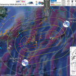
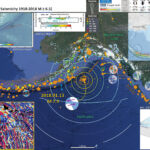
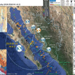
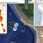
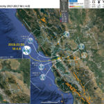
Good Morning Humboldt County!
I was in bed checking up on social media stuff and I checked my email. There were two emails from USGS ENS showing a M 5.0 near me. I had not felt it and when I went to the USGS websites, the event had been deleted. However, when i returned to twitter, I noticed @Allomax had tweeted about a M 5.7 on the Mendocino fault. So, I got out of bed and made some coffee (half decaf). It has been a busy January (lots of earthquakes).
Today’s M 5.8 earthquake happened along the Mendocino fault zone, very close to the 1994 M 7.1 epicenter. Given this being an offshore location, the location uncertainty with those settings, these may have both happened in the same location.
Today’s M 5.8 earthquake was along the western part of the Mendocino fault (MF), a right-lateral (dextral) transform plate boundary. This plate boundary connects the Gorda ridge and Juan de Fuca rise spreading centers with their counterparts in the Gulf of California, with the San Andreas strike-slip fault system. Transform plate boundaries are defined that they are strike-slip and that they connect spreading ridges. In this sense of the definition, the Mendocino fault and the San Andreas fault are part of the same system. Here is the USGS website for this earthquake.
See the figures from Rollins and Stein (2010) below. More on earthquakes in this region can be found in Earthquake Reports listed at the bottom of this page above the appendices.
The San Andreas fault is a right-lateral strike-slip transform plate boundary between the Pacific and North America plates. The plate boundary is composed of faults that are parallel to sub-parallel to the SAF and extend from the west coast of CA to the Wasatch fault (WF) system in central Utah (the WF runs through Salt Lake City and is expressed by the mountain range on the east side of the basin that Salt Lake City is built within).
The three main faults in the region north of San Francisco are the SAF, the MF, and the Bartlett Springs fault (BSF). I also place a graphical depiction of the USGS moment tensor for this fault. The SAF, MF, and BSF are all right lateral strike-slip fault systems. There are no active faults mapped in the region of Sunday’s epicenter, but I interpret this earthquake to have right-lateral slip. Without more seismicity or mapped faults to suggest otherwise, this is a reasonable interpretation.
The Cascadia subduction zone is a convergent plate boundary where the Juan de Fuca and Gorda plates (JDFP and GP, respectively) subduct norteastwardly beneath the North America plate at rates ranging from 29- to 45-mm/yr. The Juan de Fuca and Gorda plates are formed at the Juan de Fuca Ridge and Gorda Rise spreading centers respectively. More about the CSZ can be found here.
There was a good sized (M 6.5) MF earthquake late in 2016 2016.12.08. I present my poster for that earthquake below. Here is my report for that earthquake. Here is the updated report.
There was also a M 5.7 earthquake in 2017 (2017.09.22). Here is my report for that earthquake.

Below is my interpretive poster for this earthquake

I plot the seismicity from the past month, with color representing depth and diameter representing magnitude (see legend). I include earthquake epicenters from 1918-2018 with magnitudes M ≥ 5.5.
I plot the USGS fault plane solutions (moment tensors in blue and focal mechanisms in orange) for the M 5.8 earthquake, in addition to the 1994 Mendocino fault earthquake.

  • I placed a moment tensor / focal mechanism legend on the poster. There is more material from the USGS web sites about moment tensors and focal mechanisms (the beach ball symbols). Both moment tensors and focal mechanisms are solutions to seismologic data that reveal two possible interpretations for fault orientation and sense of motion. One must use other information, like the regional tectonics, to interpret which of the two possibilities is more likely.
  • I also include the shaking intensity contours on the map. These use the Modified Mercalli Intensity Scale (MMI; see the legend on the map). This is based upon a computer model estimate of ground motions, different from the “Did You Feel It?” estimate of ground motions that is actually based on real observations. The MMI is a qualitative measure of shaking intensity. More on the MMI scale can be found here and here. This is based upon a computer model estimate of ground motions, different from the “Did You Feel It?” estimate of ground motions that is actually based on real observations.
  • I include the slab contours plotted (Hayes et al., 2012), which are contours that represent the depth to the subduction zone fault. These are mostly based upon seismicity. The depths of the earthquakes have considerable error and do not all occur along the subduction zone faults, so these slab contours are simply the best estimate for the location of the fault.
  • I include some inset figures.

  • In the upper right corner is a map of the Cascadia subduction zone (CSZ) and regional tectonic plate boundary faults. This is modified from several sources (Chaytor et al., 2004; Nelson et al., 2004). I placed a blue star in the general location of today’s M 5.7 earthquake.
  • Below the CSZ map is an illustration modified from Plafker (1972). This figure shows how a subduction zone deforms between (interseismic) and during (coseismic) earthquakes. Today’s earthquake did not occur along the CSZ, so did not produce crustal deformation like this. However, it is useful to know this when studying the CSZ.
  • In the lower left corner is a figure from Rollins and Stein (2010). In their paper they discuss how static coulomb stress changes from earthquakes may impart (or remove) stress from adjacent crust/faults. This map shows the major earthquakes that have occurred in this region, prior to their publication in 2010. I place a blue star in the general location of today’s earthquake.
  • In the upper left corner is a map showing historic focal mechanisms along the MF (Dengler et al., 1995). This figure shows how the GPS sites moved during that earthquake, showing that the CSZ megathrust fault is seismologically coupled.


  • This is the report from my DYFI submission.


Some Relevant Discussion and Figures

  • Here is a map from Rollins and Stein, showing their interpretations of different historic earthquakes in the region. This was published in response to the January 2010 Gorda plate earthquake. The faults are from Chaytor et al. (2004). The 1980, 1992, 1994, 2005, and 2010 earthquakes are plotted and labeled. I did not mention the 2010 earthquake, but it most likely was just like 1980 and 2005, a left-lateral strike-slip earthquake on a northeast striking fault.

  • Tectonic configuration of the Gorda deformation zone and locations and source models for 1976–2010 M ≥ 5.9 earthquakes. Letters designate chronological order of earthquakes (Table 1 and Appendix A). Plate motion vectors relative to the Pacific Plate (gray arrows in main diagram) are from Wilson [1989], with Cande and Kent’s [1995] timescale correction.

  • Here is the Rollins and Stein (2010) figure that is in the report above. I include their figure caption as blockquote below.

  • Coulomb stress changes imparted by our models of (a) a bilateral rupture and (b) a unilateral eastward rupture for the 1994 Mw = 7.0 Mendocino Fault Zone earthquake to the epicenters of the 1995 Mw = 6.6 southern Gorda zone earthquake (N) and the 2000 Mw = 5.9 Mendocino Fault Zone earthquake (O). Calculation depth is 5 km.

  • Here is a large scale map of the 1994 earthquake swarm. The mainshock epicenter is a black star and epicenters are denoted as white circles.

  • Here is a plot of focal mechanisms from the Dengler et al. (1995) paper in California Geology.

  • In this map below, I label a number of other significant earthquakes in this Mendocino triple junction region. Another historic right-lateral earthquake on the Mendocino fault system was in 1994. There was a series of earthquakes possibly along the easternmost section of the Mendocino fault system in late January 2015, here is my post about that earthquake series.

  • For more on the graphical representation of moment tensors and focal mechnisms, check this IRIS video out:
  • Here is a fantastic infographic from Frisch et al. (2011). This figure shows some examples of earthquakes in different plate tectonic settings, and what their fault plane solutions are. There is a cross section showing these focal mechanisms for a thrust or reverse earthquake. The upper right corner includes my favorite figure of all time. This shows the first motion (up or down) for each of the four quadrants. This figure also shows how the amplitude of the seismic waves are greatest (generally) in the middle of the quadrant and decrease to zero at the nodal planes (the boundary of each quadrant).

  • The Gorda and Juan de Fuca plates subduct beneath the North America plate to form the Cascadia subduction zone fault system. In 1992 there was a swarm of earthquakes with the magnitude Mw 7.2 Mainshock on 4/25. Initially this earthquake was interpreted to have been on the Cascadia subduction zone (CSZ). The moment tensor shows a compressional mechanism. However the two largest aftershocks on 4/26/1992 (Mw 6.5 and Mw 6.7), had strike-slip moment tensors. These two aftershocks align on what may be the eastern extension of the Mendocino fault.
  • There have been several series of intra-plate earthquakes in the Gorda plate. Two main shocks that I plot of this type of earthquake are the 1980 (Mw 7.2) and 2005 (Mw 7.2) earthquakes. I place orange lines approximately where the faults are that ruptured in 1980 and 2005. These are also plotted in the Rollins and Stein (2010) figure above. The Gorda plate is being deformed due to compression between the Pacific plate to the south and the Juan de Fuca plate to the north. Due to this north-south compression, the plate is deforming internally so that normal faults that formed at the spreading center (the Gorda Rise) are reactivated as left-lateral strike-slip faults. In 2014, there was another swarm of left-lateral earthquakes in the Gorda plate. I posted some material about the Gorda plate setting on this page.
  • There are three types of earthquakes, strike-slip, compressional (reverse or thrust, depending upon the dip of the fault), and extensional (normal). Here is are some animations of these three types of earthquake faults. Many of the earthquakes people are familiar with in the Mendocino triple junction region are either compressional or strike slip. The following three animations are from IRIS.
  • Strike Slip:

    Compressional:

    Extensional:

  • This figure shows what a transform plate boundary fault is. Looking down from outer space, the crust on either side of the fault moves side-by-side. When one is standing on the ground, on one side of the fault, looking across the fault as it moves… If the crust on the other side of the fault moves to the right, the fault is a “right lateral” strike slip fault. The Mendocino and San Andreas faults are right-lateral (dextral) strike-slip faults. I believe this is from Pearson Higher Ed.

Social Media


    References

  • Atwater, B.F., Musumi-Rokkaku, S., Satake, K., Tsuju, Y., Eueda, K., and Yamaguchi, D.K., 2005. The Orphan Tsunami of 1700—Japanese Clues to a Parent Earthquake in North America, USGS Professional Paper 1707, USGS, Reston, VA, 144 pp.
  • Chaytor, J.D., Goldfinger, C., Dziak, R.P., and Fox, C.G., 2004. Active deformation of the Gorda plate: Constraining deformation models with new geophysical data: Geology v. 32, p. 353-356.
  • Dengler, L.A., Moley, K.M., McPherson, R.C., Pasyanos, M., Dewey, J.W., and Murray, M., 1995. The September 1, 1994 Mendocino Fault Earthquake, California Geology, Marc/April 1995, p. 43-53.
  • Frisch, W., Meschede, M., Blakey, R., 2011. Plate Tectonics, Springer-Verlag, London, 213 pp.
  • Geist, E.L. and Andrews D.J., 2000. Slip rates on San Francisco Bay area faults from anelastic deformation of the continental lithosphere, Journal of Geophysical Research, v. 105, no. B11, p. 25,543-25,552.
  • Irwin, W.P., 1990. Quaternary deformation, in Wallace, R.E. (ed.), 1990, The San Andreas Fault system, California: U.S. Geological Survey Professional Paper 1515, online at: http://pubs.usgs.gov/pp/1990/1515/
  • McCrory, P.A.,. Blair, J.L., Waldhauser, F., kand Oppenheimer, D.H., 2012. Juan de Fuca slab geometry and its relation to Wadati-Benioff zone seismicity in JGR, v. 117, B09306, doi:10.1029/2012JB009407.
  • McLaughlin, R.J., Sarna-Wojcicki, A.M., Wagner, D.L., Fleck, R.J., Langenheim, V.E., Jachens, R.C., Clahan, K., and Allen, J.R., 2012. Evolution of the Rodgers Creek–Maacama right-lateral fault system and associated basins east of the northward-migrating Mendocino Triple Junction, northern California in Geosphere, v. 8, no. 2., p. 342-373.
  • Nelson, A.R., Asquith, A.C., and Grant, W.C., 2004. Great Earthquakes and Tsunamis of the Past 2000 Years at the Salmon River Estuary, Central Oregon Coast, USA: Bulletin of the Seismological Society of America, Vol. 94, No. 4, pp. 1276–1292
  • Rollins, J.C. and Stein, R.S., 2010. Coulomb stress interactions among M ≥ 5.9 earthquakes in the Gorda deformation zone and on the Mendocino Fault Zone, Cascadia subduction zone, and northern San Andreas Fault: Journal of Geophysical Research, v. 115, B12306, doi:10.1029/2009JB007117, 2010.
  • Stoffer, P.W., 2006, Where’s the San Andreas Fault? A guidebook to tracing the fault on public lands in the San Francisco Bay region: U.S. Geological Survey General Interest Publication 16, 123 p., online at http://pubs.usgs.gov/gip/2006/16/
  • Wallace, Robert E., ed., 1990, The San Andreas fault system, California: U.S. Geological Survey Professional Paper 1515, 283 p. [http://pubs.usgs.gov/pp/1988/1434/].

Earthquake Report: Gulf of Alaska UPDATE #2

UPDATES Below is a list of all the reports associated with this earthquake sequence.

I thought it would be interesting to see the seismicity with time. Perhaps this could help us learn about the fault sources associated with this earthquake sequence.
I am not sure it worked as some issues cannot be dealt with simply with this visualization.
For example, the locations for these earthquakes may not be resolute enough [yet] to figure out the orientation of the faults at work here. The back projection data are perhaps the strongest evidence for an east-west fault. However, we still have the contradictory sense of motion along the fracture zones at the meso scale… (as revealed in the EMAG2 magnetic anomaly data).
As a reminder, if the M 7.9 earthquake fault is E-W oriented, it would be left-lateral. The offset magnetic anomalies show right-lateral offset across these fracture zones. This was perhaps the main reason why I thought that the main fault was not E-W, but N-S. After a day’s worth of aftershocks, the seismicity may reveal some north-south trends. But, as a drama student in 7th grade (1977), my drama teacher (Ms. Naichbor, rest in peace) asked our class to go stand up on stage. We all stood in a line and she mentioned that this is social behavior, that people tend to stand in lines (and to avoid doing this while on stage). Later, when in college, professors often commented about how people tend to seek linear trends in data (lines). I actually see 3-4 N-S trends and ~2 E-W trends in the seismicity data.
So, that being said, here is the animation I put together. I used the USGS query tool to get earthquakes from 1/22 until now, M ≥ 1.5. I include a couple inset maps presented in my interpretive posters. The music is copyright free. The animations run through twice.
Here is a screenshot of the 14 MB video embedded below. I encourage you to view it in full screen mode (or download it).


  • Here is the seismograph at Humboldt State University, Dept. of Geology. The seismometer is located in the basement of Founders Hall, across from the Geology Dept. office.

Social Media

Earthquake Report: Gulf of Alaska UPDATE #1

Well. What a firestorm of social media discusions about this earthquake. It seems that, like how we learn so much when earthquakes like this happen, the amount of interacting in public on social media has been growing earthquake by earthquake.
I spent some time this afternoon looking at the magnetic anomalies, after taking a load of a part of an old building to the county dump (transfer station) before the rain started. Stephen Hicks found a great paper (and tweeted about it, see my original report here where I include his tweet).
UPDATES Below is a list of all the reports associated with this earthquake sequence.

In my original report, I proposed that if the earthquake happened on the USGS fault model, then there is a problem when considering the magnetic anomaly map. The USGS fault solution is left-lateral, but the magnetic anomaly offsets appear to be right-laterally offset. Upon further review, I noticed that there are some details in this area that could be interpreted as left lateral. In my poster below, I place a white arrow along the hypothetical fault (drawn as a green dashed line). I located the line based upon offsets in the magnetic anomaly data as aligned with the USGS model.
Then I took a look at the mag anomaly map from Naugler and Wageman (1973). These authors show the isochrons for the Gulf of Alaska (GA). The fracture zone nearest today’s M 7.9 earthquake is right-lateral (supporting my original interpretation). However, the USGS fault model appears to be oblique to this fracture zone. Perhaps today’s M 7.9 is on a conjugate fault, with a different sense of motion.
Interesting that the USGS fault model terminates on the eastern side with the epicenter from a 1999 earthquake. This earthquake has a fault plane solution that shows oblique slip, not pure strike-slip. This could be because (1) the earthquake happened on a different fault or (2) the earthquake happened on the same fault, but the fault is changing its orientation (I favor the first hypothesis).
Some people have been stating that the aftershocks appear to be aligned in a north-south orientation. I cannot figure out how they made this observation, but maybe I am missing something. This did make me think about instances where off fault earthquakes can be triggered, or when there are major fault systems that are not reflected in the geomorphology nor other measures of long term tectonics (like magnetic anomalies or fracture zones). A great example is the 2012 M 8.6 Wharton Basin earthquakes that ruptured in response to the 2004 Sumatra-Andaman subduction zone earthquake eight years earlier. Today’s M 7.9 earthquake is rather deep (like the 2012 earthquakes), so perhaps there are some deep faults that are not reflected by the shape of the seafloor nor reflected by the gravity data for some reason (the former seems more likely to me).

Below is my interpretive poster for this earthquake

I plot the seismicity from the past month, with color representing depth and diameter representing magnitude (see legend). I include earthquake epicenters from 1918-2018 with magnitudes M ≥ 6.5. More about the plate boundary can be found in that report.
I plot the USGS fault plane solutions (moment tensors in blue and focal mechanisms in orange) for the M 7.9 earthquake, in addition to some relevant historic earthquakes.

  • I placed a moment tensor / focal mechanism legend on the poster. There is more material from the USGS web sites about moment tensors and focal mechanisms (the beach ball symbols). Both moment tensors and focal mechanisms are solutions to seismologic data that reveal two possible interpretations for fault orientation and sense of motion. One must use other information, like the regional tectonics, to interpret which of the two possibilities is more likely.
  • I also include the shaking intensity contours on the map. These use the Modified Mercalli Intensity Scale (MMI; see the legend on the map). This is based upon a computer model estimate of ground motions, different from the “Did You Feel It?” estimate of ground motions that is actually based on real observations. The MMI is a qualitative measure of shaking intensity. More on the MMI scale can be found here and here. This is based upon a computer model estimate of ground motions, different from the “Did You Feel It?” estimate of ground motions that is actually based on real observations.
  • I include the slab contours plotted (Hayes et al., 2012), which are contours that represent the depth to the subduction zone fault. These are mostly based upon seismicity. The depths of the earthquakes have considerable error and do not all occur along the subduction zone faults, so these slab contours are simply the best estimate for the location of the fault. Slab 2.0 is due out later this year!
  • I include some inset figures.

  • In the lower right corner, I place a map from Naugler and Sageman (1973). I added relative slip vectors for the fracture zones here. I place the epicenter from today’s earthquake as a cyan star.


  • As I was rereading my report (don’t always get a chance, but good to check for typos), looking at the aftershocks, and considering the problems associated with this earthquake and its tectonic setting (i.e. right-lateral fracture zones and a left-lateral USGS fault solution), I decided to make some updates to this large scale poster. There were several aftershocks while I was making this map that made a north-south trend more apparent. So, now I am favoring the following interpretation: the M 7.9 mainshock and many aftershocks are the result of a right-lateral north-striking strike-slip fault.
  • This is the exact same thing that happened following the 2012 Wharton Basin M 8.6/8.2 earthquake sequence along the outer rise of the Sumatra-Andaman subduction zone. The M 8.6 is the largest strike-slip intraplate earthquake ever recorded on modern seismometers. I present some maps from Sumatra earthquakes below. Basically, the fracture zones in the the India-Australia plate trend north-south. So that was my initial interpretation, that these earthquakes were left-lateral earthquakes on faults associated with these fracture zones. However, this was not the case. The Wharton Basin earthquake sequence involved both fracture zone related faults, in addition to conjugate faults trending east-west. There were initially fault slip models for both interpretations.


Some Relevant Discussion and Figures

  • This is a great map from UNAVCO. This shows the static offsets to GPS sites as a result of this M 7.9 earthquake.

  • Seismically derived static displacements (first figure, pink is p1 and blue is p2) and their difference (figure 2)(Figure/Dave Mencin, UNAVCO)

  • Here are some interpretive posters from the 2012 Sumatra Outer Rise earthquake sequence.
  • I have presented materials related to the 2004 Sumatra-Andaman subduction zone earthquake here and more here.
  • I include a map in the upper right corner that shows the historic earthquake rupture areas. There is a figure from Meng et al. (2012) that shows the details about the faults and the seismicity.

  • Here is that Meng et al. (2012) figure showing the different faults that ruptured in 2012.

  • Here is a poster that shows some earthquakes in the Andaman Sea. This is from my earthquake report from 2015.11.08.

  • This map shows the fracture zones in the India-Australia plate.

Review Stuff from my first report.

  • Here is a map for the earthquakes of magnitude greater than or equal to M 7.0 between 1900 and 2016. This is the USGS query that I used to make this map. One may locate the USGS web pages for all the earthquakes on this map by following that link.

Social Media

Earthquake Report: Gulf of Alaska!

I was asleep in bed, trying to catch up to prevent myself from getting ill, when there was a large earthquake in the Gulf of Alaska (GA), offshore of Kodiak, Alaska. When I wakened, I noticed a fb message from my friend Scott Willits notifying me of an M 8.2 earthquake in Alaska, posted at 2:20 AM local time. I immediately got up to check on this and was surprised that there was not a tsunami evacuation going on. I live in the small town of Manila (population ~700), on the North Spit (a sand spit west of Arcata and Eureka, CA). I live above 10 m in elevation and do not consider myself exposed to tsunami risks, local or distant (especially given that (1) the CSZ locked zone is mostly under land here and (2) that the part of the locked zone that is not under land is in shallow water; so our local tsunami will probably be much smaller than further north, like Crescent City or Brookings). I have been involved in tsunami education and outreach for over 15 years and prepared the first tsunami hazard map for northern CA (working with Dr. Lori Dengler and the Redwood Coast Tsunami Work Group). Needless to say, I am cogent and aware about the tsunami risk here in norcal.

https://earthquake.usgs.gov/earthquakes/eventpage/us2000cmy3/executive

SO. I soon discovered that the GA earthquake happened in the Pacific plate, far from the subduction zone and that the earthquake was a strike-slip earthquake. Both of these facts explained why the sheriff had not been at my door earlier this morning. In addition, the magnitude had been adjusted to M 7.9 (no longer a Great earthquake, just a Large earthquake; earthquake classes are defined here). However, there were some small tsunami waves observed (see below) as reported by the National Tsunami Warning Center (see social media below).
This earthquake appears to be located along a reactivated fracture zone in the GA. There have only been a couple earthquakes in this region in the past century, one an M 6.0 to the east (though this M 6.0 was a thrust earthquake). The Gulf of Alaska shear zone is even further to the east and has a more active historic fault history (a pair of earthquakes in 1987-1988). The magnetic anomalies (formed when the Earth’s magnetic polarity flips) reflect a ~north-south oriented spreading ridge (the anomalies are oriented north-south in the region of today’s earthquake). There is a right-lateral offset of these magnetic anomalies located near the M 7.9 epicenter. Interesting that this right-lateral strike-slip fault (?) is also located at the intersection of the Gulf of Alaska shear zone and the 1988 M 7.8 earthquake (probably just a coincidence?). However, the 1988 M 7.8 earthquake fault plane solution can be interpreted for both fault planes (it is probably on the GA shear zone, but I don’t think that we can really tell).
This is strange because the USGS fault plane is oriented east-west, leading us to interpret the fault plane solution (moment tensor or focal mechanism) as a left-lateral strike-slip earthquake. So, maybe this earthquake is a little more complicated than first presumed. The USGS fault model is constrained by seismic waves, so this is probably the correct fault (east-west).
I prepared an Earthquake Report for the 1964 Good Friday Earthquake here.
UPDATES Below is a list of all the reports associated with this earthquake sequence.

Below is my interpretive poster for this earthquake

I plot the seismicity from the past month, with color representing depth and diameter representing magnitude (see legend). I include earthquake epicenters from 1918-2018 with magnitudes M ≥ 6.5. More about the plate boundary can be found in that report.
I plot the USGS fault plane solutions (moment tensors in blue and focal mechanisms in orange) for the M 7.9 earthquake, in addition to some relevant historic earthquakes.

  • I placed a moment tensor / focal mechanism legend on the poster. There is more material from the USGS web sites about moment tensors and focal mechanisms (the beach ball symbols). Both moment tensors and focal mechanisms are solutions to seismologic data that reveal two possible interpretations for fault orientation and sense of motion. One must use other information, like the regional tectonics, to interpret which of the two possibilities is more likely.
  • I also include the shaking intensity contours on the map. These use the Modified Mercalli Intensity Scale (MMI; see the legend on the map). This is based upon a computer model estimate of ground motions, different from the “Did You Feel It?” estimate of ground motions that is actually based on real observations. The MMI is a qualitative measure of shaking intensity. More on the MMI scale can be found here and here. This is based upon a computer model estimate of ground motions, different from the “Did You Feel It?” estimate of ground motions that is actually based on real observations.
  • I include the slab contours plotted (Hayes et al., 2012), which are contours that represent the depth to the subduction zone fault. These are mostly based upon seismicity. The depths of the earthquakes have considerable error and do not all occur along the subduction zone faults, so these slab contours are simply the best estimate for the location of the fault. Slab 2.0 is due out later this year!
  • I include some inset figures.

  • In the upper left corner, I place a map created by Dr. Peter Haeussler, USGS, which shows the historic earthquakes along the Alaska and Aleutian subduction zones. I place the epicenter from today’s earthquake as a cyan star.
  • To the right of this map, I include first the USGS map that shows their interpretation of where the fault is (the red line) and then I include the USGS fault slip model (color = slip in meters).
  • In the upper right corner is a map from IRIS that shows seismicity with color representing depth.
  • In the lower right corner, I include a low angle oblique view of the subduction zone, showing how the Pacific plate is subducting beneath the North America plate.
  • In the lower left corner, I include a map that shows the magnetic anomalies in the GA region. I include USGS seismicity from 1918-2018 for earthquakes M ≥ 5.5.


  • UPDATE 12:45 my local time
  • The USGS updated their MMI contours to reflect their fault model. Below is my updated poster. I also added green dashed lines for the fracture zones related to today’s M 7.9 earthquake (on the magnetic anomaly inset map).


  • These are the observations as reported by the NTWC this morning (at 4:15 AM my local time).

  • Here is an educational video from IRIS about the tectonics in Alaska.

Some Relevant Discussion and Figures

  • Here is a map for the earthquakes of magnitude greater than or equal to M 7.0 between 1900 and 2016. This is the USGS query that I used to make this map. One may locate the USGS web pages for all the earthquakes on this map by following that link.

  • Here is a cross section showing the differences of vertical deformation between the coseismic (during the earthquake) and interseismic (between earthquakes).

  • Here is a figure recently published in the 5th International Conference of IGCP 588 by the Division of Geological and Geophysical Surveys, Dept. of Natural Resources, State of Alaska (State of Alaska, 2015). This is derived from a figure published originally by Plafker (1969). There is a cross section included that shows how the slip was distributed along upper plate faults (e.g. the Patton Bay and Middleton Island faults).

  • There are three types of earthquakes, strike-slip, compressional (reverse or thrust, depending upon the dip of the fault), and extensional (normal). Here is are some animations of these three types of earthquake faults. Many of the earthquakes people are familiar with in the Mendocino triple junction region are either compressional or strike slip. The following three animations are from IRIS.
  • Strike Slip:
  • Compressional:
  • Extensional:
  • This figure shows what a transform plate boundary fault is. Looking down from outer space, the crust on either side of the fault moves side-by-side. When one is standing on the ground, on one side of the fault, looking across the fault as it moves… If the crust on the other side of the fault moves to the right, the fault is a “right lateral” strike slip fault. The Mendocino and San Andreas faults are right-lateral (dextral) strike-slip faults. I believe this is from Pearson Higher Ed.

  • For more on the graphical representation of moment tensors and focal mechnisms, check this IRIS video out:
  • Here is a fantastic infographic from Frisch et al. (2011). This figure shows some examples of earthquakes in different plate tectonic settings, and what their fault plane solutions are. There is a cross section showing these focal mechanisms for a thrust or reverse earthquake. The upper right corner includes my favorite figure of all time. This shows the first motion (up or down) for each of the four quadrants. This figure also shows how the amplitude of the seismic waves are greatest (generally) in the middle of the quadrant and decrease to zero at the nodal planes (the boundary of each quadrant).

Social Media

Earthquake Report: Gulf of California

Today we had an earthquake with magnitude M 6.3 in the Gulf of California (GOC). The GOC is formed by transtension (extension along a strike-slip fault system) along the North-America-Pacific plate boundary. Transtension happens when the plate motion across a fault is not oriented parallel to the fault. This non-optimal relation (plate motion vs fault direction) can generally happen as a result of (1) a bending fault or (2) due to stepped offsets of the fault. The dextral (right-lateral) strike-slip faults here make “right-steps” and pull apart basins form in these locations.
The strike-slip faults are offset by oceanic spreading ridges. These spreading ridges are connected the East Pacific Rise to the south (and the Juan de Fuca Ridge and Gorda Rise to the north, via the San Andreas fault).
The geology of this region is much more complicated than this, but this is a good place to start when trying to understand the tectonics here. This M 6.3 earthquake happened on the southern boundary of the Guamas Basin, one of these pull apart basins.
So far there has been a single aftershock (M 4.5).
This M 6.3 earthquake appears to be pretty typical of this part of the Gulf. There have been several M 6 earthquakes in the last century. There have been a couple M 7 earthquakes, to the north.

Below is my interpretive poster for this earthquake

I plot the seismicity from the past month, with color representing depth and diameter representing magnitude (see legend). I include earthquake epicenters from 1918-2018 with magnitudes M ≥ 6.5.
I plot the USGS fault plane solutions (moment tensors in blue and focal mechanisms in orange) for the M 6.3 earthquakes, in addition to some relevant historic earthquakes.
I labeled the pull-apart basins in cyan and the faults in light orange. CdBF – C. de Ballenas fault; GF – Guaymas fault; CF – Carmen fault; FF – Farallon fault; PF – Pescadero fault; AF – Alcaron fault; AR – Alcaron Ridge (from Aragón-Arreola, M. and Martín-Barajas, A., 2007).

  • I placed a moment tensor / focal mechanism legend on the poster. There is more material from the USGS web sites about moment tensors and focal mechanisms (the beach ball symbols). Both moment tensors and focal mechanisms are solutions to seismologic data that reveal two possible interpretations for fault orientation and sense of motion. One must use other information, like the regional tectonics, to interpret which of the two possibilities is more likely.
  • I also include the shaking intensity contours on the map. These use the Modified Mercalli Intensity Scale (MMI; see the legend on the map). This is based upon a computer model estimate of ground motions, different from the “Did You Feel It?” estimate of ground motions that is actually based on real observations. The MMI is a qualitative measure of shaking intensity. More on the MMI scale can be found here and here. This is based upon a computer model estimate of ground motions, different from the “Did You Feel It?” estimate of ground motions that is actually based on real observations.

    I include some inset figures.

  • In the lower left corner I include a map that shows the tectonic setting of this region, with the geological units colored relative to their age and type (marine or continental). This is from a paper that discusses the interaction between spreading ridges and subduction trenches (Fletcher et al., 2007). I place a blue star in the general location of today’s earthquake.
  • In the upper left corner is the plate tectonic history for the past 12.3 Ma from Fletcher et al. (2007). I place a blue star in the general location of today’s earthquake.
  • Between the 2 Fletcher et al. (2007) figures is a figure that shows how there can be extension and compression along strike-slip figures.
  • Along the right side is the tectonic history of the GOC as interpreted by Bennett et al. (2013). I place a blue star in the general location of today’s earthquake. I used to think that the spreading ridges in the GOC were from the ridge that originally formed the Farallon plate. However, I have learned that the GOC extension formed as a result of the misfit of the plate boundary relative to plate motions (causing transtension).


  • On 2017.03.29 there was an M 5.7 earthquake in this same region as today’s M 6.3 earthquake. Here is my report and below is my interpretive poster.

  • There was an earthquake on 2015.09.13 (M 6.6) located in the area of the Farallon Basin (here is my earthquake report page and the update page). Below is a map I prepared that shows the general location of the pull-apart basins along this plate boundary.

  • Here is a fantastic animation showing the tectonic history of the GOC for the past 11 million years (Bennet et al., 2016). This animation was created using existing geological maps and fault data (geometry, changing or static slip-rates) and backing out the motion on the faults to create a map of what the geology looked like in the past.
  • There are several ways to do this and Bennett et al. (2016) use a Palinspastic reconstruction technique. These authors hypothesize that, based upon their observations, the transtension along this plate boundary promoted subsidence in the GOC. Read more about the Colorado River and how it responded to this tectonic forcing in their paper.

  • This is the Bennet et al. (2013) figure from the poster, which shows their interpretation for the tectonic history of the GOC. This is based largely on their tectonic reconstructions in the northern GOC.

  • Modified integrated transtensional shear model for the tectonic evolution of the Gulf of California. North America plate fixed. (A) Prior to 28 Ma, the spreading center between Pacific and Vancouver-Farallon tectonic plates approached the subduction zone between North America and Vancouver-Farallon plates. (B) By ca. 20 Ma, contact between the Pacific and North America plates created early dextral transform relative plate motion. The Basin and Range extensional province (light gray) accommodated moderate extension throughout western North America. (C) The Rivera triple junction migrated the full length of the Baja California Peninsula by ca. 12.5 Ma, lengthening the Pacific–North American transform plate boundary. The proto–Gulf of California period commenced (ca.12.5 Ma) with transtensional strain distributed across two distinct transtensional deformation belts, west and east of the stable Baja California microplate. (D) In late proto–Gulf of California time, shear deformation gradually localized within a narrow belt of focused en- echelon dextral shear zones embedded within the greater Mexican Basin and Range extensional province. These shear zones and intervening extensional regions both experienced high-magnitude strain. (E) By ca. 6 Ma, Pacific–North America plate boundary strain was localized and focused crustal thinning and subsidence in transtensional pull-apart basins that formed the Gulf of California. Faults shown represent primary structures active during Quaternary time. RP—Rivera plate, JDFP—Juan de Fuca plate, RTJ—Rivera triple junction, MTJ—Mendocino triple junction, SAF— San Andreas fault, CP—Colorado Plateau, SMO—Sierra Madre Occidental.

  • This is the Sutherland et al. (2012) interpretation of the geological history for the plate boundary in this region. These authors used seismic reflection data (multi-channel seismic) from a profile oriented parallel to the Alarcón Basin (perpendicular to the spreading ridge).

  • The model for the tectonic evolution of the Gulf of California (GOC). (A) The starting point of the evolution of the GOC began 14–12 Ma, where the Magdalena rise stalled off the west coast of Baja California; there was also a marked changed in the style of volcanism. Plate motion was split between the dying spreading ridge, subduction zone, and the new highly oblique extension in the proto–GOC. During this time, the dipping part of the subducted plate appears to have broken off, opening a slab window beneath the southern Baja peninsula. NAM—North American plate; PAC—Pacific plate. (B) Another major change in the system occurs near 8–7 Ma, where the volcanic style changes once again with many lavas of unusual composition deposited. Any minor component of spreading finally ceases and the Tosco-Abreojos fault forms within the borderlands west of Baja. Oblique extension continues in the GOC. (C) Seafloor spreading begins at the Alarcón Rise between 4 and 3 Ma. Small amounts of movement continue along the Tosco-Abreojos fault (TAF); even today the Baja peninsula is not fully transferred to the Pacific plate.

  • This shows the location of the Sutherland et al. (2012) seismic reflection profile.

  • Map showing location of Alarcón transect and the major basins along the profile.

  • This is the overview of the Sutherland et al. (2012) seismic reflection data.

  • An overview of multichannel seismic transect data presented in this paper. Seismic data are post-stack time migrated. TWTT—two-way travel time.

  • This is an example of the Sutherland et al. (2012) seismic reflection data, showing their interpretation in the lower panel. Note the extensive normal (and perhaps strike-slip) faulting (remember, we are in an extensional basin).

  • East Cerralvo basin. The uninterpreted (top) and interpreted (bottom) seismic profi les are shown. TWTT—two-way traveltime. Basement reflections are highlighted in blue, and sedimentary sequence boundaries are separated by green lines, with faults shown in red. Basement has a reflective discontinuous appearance. Unit 1 (divided into 1a and 1b) is a synrift deposit, with a chaotic character; unit 2 (divided into 2a and 2b) exhibits rotation and divergence and appears to be synrift; unit 3 consists of postrift, layered deeper water marine sediments. Two surface-cutting normal faults at the southeast end appear younger than the main basin, although the exact relationship of faulting is unclear and they appear to be overprinted by current-controlled erosion.

  • Here is a great diagram showing the major faults in the region (Umhoefer et al., 2002). I include their figure caption below.

  • (A) Simplified map of the Gulf of California region and Baja California peninsula showing the present plate boundary and some major tectonic features related to the plate-tectonic history since 12 Ma. The Gulf extensional province in gray is bounded by the Main Gulf Escarpment (bold dashed lines), which runs through the Loreto area and is shown in Figure 3. The Salton trough in southern California is merely the northern part of the Gulf extensional province. (B) Map of part of the southern Gulf of California and Baja California peninsula showing bathymetry (in meters), the transform–spreading-ridge plate boundary, and the location of subsequent figures with maps. The bathymetry is after a map in Ness and Lyle (1991) and the transform–spreading-ridge plate boundary is from Lonsdale (1989). The lines with double arrows are the three proposed rift segments modified here after Axen (1995); MS—Mulege´ segment, LS—Loreto segment, TS—Timbabichi
    segment.

  • This map shows the magnetic anomalies and the geologic map for the land and the youngest oceanic crust.

  • (A) Tectonic map of the southern Baja California microplate (BCM) and Gulf of California extensional province (GEP). The Magdalena fan is deposited on oceanic crust of the Farallon-derived Magdalena microplate located west of Baja California. Deep Sea Drilling Project Site 471 is shown as black dot on the Magdalena fan. Abbreviations: BCT—Baja California trench, BM—Bahia Magdalena, LC—Los Cabos block, T—Trinidad block, LP—La Paz, PV—Puerto Vallarta, SMSLF—Santa Margarita–San Lazaro fault, TAF—Tosco-Abreojos fault, TS—Todos Santos, V—Vizcaino peninsula. Geology is simplifi ed from Muehlberger (1996). Interpretation of marine magnetic anomalies, with numbers denoting the chron of positively magnetized stripes, is from Severinghaus and Atwater (1989) and Lonsdale (1991).

  • This map shows a more broad view of the magnetic anomalies through time.

  • Map-view time slices showing the widely accepted model for the two-phase kinematic evolution of plate margin shearing around the Baja California microplate. (A) Configuration of active ridge segments (pink) west of Baja California just before they became largely abandoned ca. 12.3 Ma. (B) It is thought that plate motion from 12.3 to 6 Ma was kinematically partitioned into dextral strike slip (325 km) on faults west of Baja California and orthogonal rifting in the Gulf of California (90 km). This is known as the protogulf phase of rifting. (C) From 6 to 0 Ma faults west of Baja California are thought to have died and all plate motion was localized in the Gulf of California, which accommodated ~345 km of integrated transtensional shearing. Despite its wide acceptance, our data preclude this kinematic model. In all frames, the modern coastline is blue. Continental crust that accommodated post–12.3 Ma shearing is dark brown. Unfaulted microplates of continental crust are light tan. Farallon-derived microplates are light green. Middle Miocene trench-filling deposits like the Magdalena fan are colored dark green. Deep Sea Drilling Project Site 471 is the black dot on the southern Magdalena microplate. Yellow line (296 km) in the northern Gulf of California connects correlated terranes of Oskin and Stock (2003). Maps have Universal Transverse Mercator zone 12 projection with mainland Mexico fixed in present position.

  • This is a nice simple figure, from the University of Sydney here, showing the terminology of strike slip faulting. It may help with the following figures.
  • Here is a fault block diagram showing how strike-slip step overs can create localized compression (positive flower) or extension (negative flower). More on strike-slip tectonics (and the source of this image) here.

  • This is an animation from Tanya Atwater. Click on this link to take you to yt (if the embedded video below does not work).

Update

  • I just found a paper that includes a map of the pull-apart basins in the northern GOC (Aragón-Arreola and Martín-Barajas, 2007). Today’s M 6.3 earthquake happened along the Carmen fault zone (labelled 11), close to where the letter L is located..

  • Eastern Gulf of California contains abandoned rift basins, while active rifting occurs in the western Gulf (Lonsdale, 1989; Fenby and Gastil, 1991; Persaud et al., 2003; Aragón-Arreola et al., 2005; this study). Eastern Gulf constitutes abandoned rift margin (see inset). PA—Pacifi c plate; GC—Gulf of California; GEP—Gulf Extensional Province; B&R—Basin
    and Range Province; SMO—Sierra Madre Occidental; CP—Colorado Plateau: ITI—Isla Tiburón; IAG—Isla Ángel de la Guarda.

References:

Earthquake Report: Peru Update #1

Well, I missed looking further into a key update paper and used figures from an older paper on my interpretive poster yesterday. Thanks to Stéphane Baize for pointing this out! Turns out, after their new analyses, the M 7.1 earthquake was in a region of higher seismogenic coupling, rather than low coupling (as was presented in my first poster).
Also, Dr. Robin Lacassin noticed (as did I) the paucity of aftershocks from yesterday’s M 7.1. This was also the case for the carbon copy 2013 M 7.1 earthquake (there was 1 M 4.6 aftershock in the weeks following the M 7.1 earthquake on 2013.09.25; there were a dozen M 1-2 earthquakes in Nov. and Dec. of 2013, but I am not sure how related they are to the M 7.1 then). I present a poster below with this in mind. I also include below a comparison of the MMI modeled estimates. The 2013 seems to have possibly generated more widespread intensities, even though that was a deeper earthquake.

Below is my interpretive poster for this earthquake

I plot USGS seismicity from 2013.09.24 through 2014.01.26 (about 3 months), in addition to the 2018.01.14 M 7.1 earthquake.

  • I placed a moment tensor / focal mechanism legend on the poster. There is more material from the USGS web sites about moment tensors and focal mechanisms (the beach ball symbols). Both moment tensors and focal mechanisms are solutions to seismologic data that reveal two possible interpretations for fault orientation and sense of motion. One must use other information, like the regional tectonics, to interpret which of the two possibilities is more likely.
  • I include the slab contours plotted (Hayes et al., 2012), which are contours that represent the depth to the subduction zone fault. These are mostly based upon seismicity. The depths of the earthquakes have considerable error and do not all occur along the subduction zone faults, so these slab contours are simply the best estimate for the location of the fault. However, we must await slab v 2.0 to get a better view of these slab contours in this region.
  • I include some inset figures.

  • In the upper right corner is an updated time-space figure (showing along-strike lengths for historic earthquakes), along with slip patches for some of these earthquakes (Villegas-Lanza et al., 2016). I place a blue star in the general location of the 2018.01.14 M 7.1 earthquake.
  • This is the updated seismic coupling figure from Villegas-Lanza et al. (2016). I place a blue star in the general location of the 2018.01.14 M 7.1 earthquake. Note how this M 7.1 earthquake is in a region of higher coupling.


  • Here is a comparison of the intensity modeling for these comparable earthquakes. I present the intensity maps on top (with the moment tensors, labled with their strike, dip, and rake data; note how they are almost identical!), the attenuation relations in the middle (how intensity decays with distance from the earthquake), and the PAGER alerts at the bottom. More can be found out about PAGER alerts here.

  • Here is the Villageas-Lanza et al. (2016) figure 1, showing their time-space diagram, along with the historic earthquake limits and patches.

  • (a) Seismotectonic setting of the South American subduction zone. The red ellipses indicate the approximate rupture areas of large subduction earthquakes (M≥ 7.5) between 1868 and 2015 [Silgado, 1978; Beck and Ruff, 1989; Dorbath et al., 1990; Beck et al., 1998]. The blue ellipses indicate the locations of moderate tsunami-earthquakes [Pelayo and Wiens, 1990; Ihmle et al., 1998]. The bathymetry from GEBCO30s highlights the main tectonic structures of the subducting Nazca Plate, which are from north to south: Carnegie Ridge (CR), Grijalva Ridge (GR), Alvarado Ridge (AR), Sarmiento Ridge (SR), Virú Fracture Zone (VFZ), Mendaña Fracture Zone (MFZ), Nazca Ridge (NR), Nazca Fracture Zone (NFZ), Iquique Ridge, Juan Fernandez Ridge, Challenger Fracture Zone (CFZ), and Mocha Fracture Zone (MCFZ). The white arrow indicates the convergence of the Nazca Plate relative to the stable South America (SSA) reference frame [Kendrick et al., 2003]. The slab geometry isodepth contours are reported every 50 km (solid lines) and 10 km (dashed lines), based on the Slab1.0 model [Hayes et al., 2012]. The dashed rectangle corresponds to Figures 1b and 1c. The N.A.S. and C.A.S. labels indicate the North Andean and the Central Andes Slivers [Bird, 2003], respectively. (b) Temporal and spatial distributions of large subduction earthquakes with Mw ≥ 7.5 that occurred in Peru since the sixteenth century. The rupture extent values (in km) of historical (gray) and recent (red) megathrust earthquakes along the Peruvian margin are shown as a function of time (in years). A triangle indicates if a tsunami was associated with the event. The orange bands denote the entrance of the NR and the MFZ delimiting the northern, central, and southern Peru subduction segments. The rupture lengths were taken from its corresponding published slip models [Silgado, 1978; Beck and Ruff, 1989; Dorbath et al., 1990; Pelayo and Wiens, 1990; Ihmle et al., 1998; Giovanni et al., 2002; Salichon et al., 2003; Pritchard et al., 2007; Bilek, 2010; Delouis et al., 2010; Moreno et al., 2010; Schurr et al., 2014], and for historical earthquakes, we estimated its approximated lengths using scaling law relationships [Wells and Coppersmith, 1994]. (c) A map of the rupture areas of large subduction earthquakes that occurred in the twentieth century [Silgado, 1978; Beck and Ruff, 1989; Dorbath et al., 1990; Ihmle et al., 1998; Giovanni et al., 2002; Sladen et al., 2010; Chlieh et al., 2011], with their associated gCMT focal mechanisms. In northern Peru, the 1960 (Mw = 7.6) Piura earthquake and the 1996 (Mw = 7.5) Chimbote earthquake, which are shown by cyan-colored polygons, were identified as tsunami-earthquake events [Pelayo and Wiens, 1990; Ihmle et al., 1998; Bilek, 2010].

  • Here is a figure from Villegas-Lanza et al. (2016) that shows the along-strike variation in moment deficit. Moment deficit is the amount of energy absorbed into the tectonic system, from plate motions, that is stored as seismic strain to be released during earthquakes. Regions where the fault is slipping freely (aseismic), seismic moment does not accumulate, so there is no moment deficit there (e.g. along the subduction zone where the Nazca Ridge intersects the megathrust). The two panels on the right are their minimum and maximum seismogenic coupling maps (showing the end members of their models). I explain the coupling ratio (0-1, white to red in color) on my initial earthquake report.
  • The key update in this paper (an update to the Chlieh et al., 2011 results) is that these authors treated the accretionary part of the South America plate as an independent player, as a forearc sliver (sort of like a microplate)

  • (left) Along-trench variations of moment deficit rate for (middle) minimum and (right) maximum interseismic coupling models. Even though the interseismic pattern might vary significantly between models, the locations of the peaks and valleys in the rate of moment deficit are very persistent characteristics that highlight the locations of the principal asperities (peaks) and creeping barriers (valleys). The dashed ellipse contours in the middle map show the approximate rupture area of large earthquakes, as described in Figure 1. (see above, the time-space figure)

  • Here is the Chlieh et al. (2011) version of this figure for comparison.
  • This is the figure that adds moment deficit to the seismic moment plot and the coupling ratio to the slip patch map.

  • Comparison of interseismic coupling along the megathrust with ruptures of large megathrust earthquakes in central and southern Peru. (left) Interseismic coupling map for 3-plate model Short4; it indicates that where the Nazca ridge and the Nazca fracture zone subduct, the interseismic coupling is low. The largest earthquake there is the Mw8.1–8.2 earthquake of 1942. It is not clear whether the 1942 rupture propagated through the Nazca ridge or stopped south of it. High interseismic coupling patches correlate well with regions that experienced great megathrust earthquake Mw8.8 in 1868 and Mw8.6–8.8 in 1746. In the south, the presence of two wide asperities separated by a wide aseismic patch may explain partially the seismic behavior of this segment in the last centuries. Individual ruptures of these asperities would produce Mw8 events, as in 2001, but their simultaneous rupture could generate great Mw > 8.5 earthquakes as in 1604 or 1868. The along-strike coincidence of the high coupling areas (orange-red) with the region of high coseismic slip during the 2001 Arequipa and 2007 Pisco earthquakes suggests that strongly coupled patches during the interseismic period may indicate the location of future seismic asperities. (right) Moment deficit (dashed lines) since the last great earthquake of 1868, 1942 and 1746 compared with the seismic moment released during recent and historical earthquakes of Figure 8. The moment deficit is computed from the rate of moment deficit predicted by model Short4 considering a steady state interseismic process (Max) or 50% of it (Min) to account for time-variable interseismic process and transient events.

  • Here is an updated moment deficit figure for this part of the Peru-Chile trench (Villegas-Lanza et al., 2016). I include the Chlieh et al. (2011) figure for comparison.
  • Chlieh et al., 2011
  • This figure shows their results used to show how different parts of the subduction zone have higher or lower moment deficits. The Central Peru section shows that there is an unmet interseismic deficit, while the southern Peru profile shows that earthquakes have been keeping up with plate convergence here. The central Peru region is the region of the subduction zone shown in the 2 figures above this one (Arica, Peru is the southern boundary between the central and southern Peru regions of this subduction zone).

  • Cumulative deficit of moment and seismic moment released due to major subduction earthquakes since the 16th century (top) in central Peru and (bottom) in southern Peru. The cumulative deficit of moment is predicted from the rates of 3-plate models Short4 in central Peru and Short10 in southern Peru (Table 5 and Figure 4). The uncertainties of moment released by historical events lead to a minimum and maximum moment released (see Table S8 in the auxiliary material). The uncertainties on the cumulative deficit of moment allow that nonlinear interseismic and viscous processes could have released 50% of the accumulated moment deficit. The remaining fraction should reflect elastic strain available to drive future earthquakes unless it would have been totally released by anelastic deformation of the forearc.

  • Villegas-Lanza et al., 2016

  • Cumulative moment deficit corrected from large earthquakes moment released since 1746, computed using the maximum, mean, and minimum interseismic models presented in Figure 6 and Table S8.

    References:

  • Antonijevic, S.K., et a;l., 2015. The role of ridges in the formation and longevity of flat slabs in Nature, v. 524, p. 212-215, doi:10.1038/nature14648
  • Bishop, B.T., Beck, S.L., Zandt, G., Wagner, L., Long, M., Knezevic Antonijevic, S., Kumar, A., and Tavera, H., 2017, Causes and consequences of flat-slab subduction in southern Peru: Geosphere, v. 13, no. 5, p. 1392–1407, doi:10.1130/GES01440.1.
  • Chlieh, M., et al., 2011. Interseismic coupling and seismic potential along the Central Andes subduction zone in JGR, v. 116, B12405, doi:10.1029/2010JB008166
  • Espurt, N., Baby, P., Brusset, S., Roddaz, M., Hermoza, W., Regard, V., Antoine, P.-O., Salas-Gismodi, R., and Bolaños, R., 2007. How does the Nazca Ridge subduction influence the modern Amazonian foreland basin? in Geology, v. 35, no. 6, p. 515-518.
  • Hayes, G. P., D. J. Wald, and R. L. Johnson, 2012. Slab1.0: A three-dimensional model of global subduction zone geometries, J. Geophys. Res., 117, B01302, doi:10.1029/2011JB008524.
  • Kumar, A., et al., 2016. Seismicity and state of stress in the central and southern Peruvian flat slab in EPSL, v. 441, p. 71-80. http://dx.doi.org/10.1016/j.epsl.2016.02.023
  • Ray., J.S., et al., 2012. Chronology and Geochemistry of Lavas from the Nazca Ridge and Easter Seamount Chain: an ~30 Myr Hotspot Record in Journal of Petrology, v. 53., no. 7, p. 1417-1448.
  • Rhea, S., Tarr, A.C., Hayes, G., Villaseñor, A., Furlong, K.P., and Benz, H.M., 2010. Seismicity of the Earth 1900-2007, Nazca plate and South America: U.S. Geological Survey Open-File Report 2010-1083-E, 1 map sheet, scale 1:12,000,000.
  • Scire, A., Zandt, G., Beck, S., Long, M., and Wagner, L., 2017, The deforming Nazca slab in the mantle transition zone and lower mantle: Constraints from teleseismic tomography on the deeply subducted slab between 6°S and 32°S: Geosphere, v. 13, no. 3, p. 665–680, doi:10.1130/GES01436.1.
  • Villegas-Lanza, J.C., et al., 2016. Active tectonics of Peru: Heterogeneous interseismic coupling along the Nazca Megathrust, rigid motion of the Peruvian Sliver and Subandean shortening accommodation in JGR, doi: 10.1002/2016JB013080

Earthquake Report: Peru

We had a damaging and (sadly) deadly earthquake in southern Peru in the last 24 hours. This is an earthquake, with magnitude M 7.1, that is associated with the subduction zone forming the Peru-Chile trench (PCT). The Nazca plate (NP) is subducting beneath the South America plate (SAP). There are lots of geologic structures on the Nazca plate that tend to affect how the subduction zone responds during earthquakes (e.g. segmentation).
In the region of this M 7.1 earthquake, two large structures in the NP are the Nazca Ridge and the Nazca fracture zone. The Nazca fracture zone is a (probably inactive) strike-slip fault system. The Nazca Ridge is an over-thickened region of the NP, thickened as the NP moved over a hotspot located near Salas y Gomez in the Pacific Ocean east of Easter Island (Ray et al., 2012).
There are many papers that discuss how the ridge affects the shape of the megathrust fault here. The main take-away is that the NR is bull dozing into South America and the dip of the subduction zone is flat here. There is a figure below that shows the deviation of the subducting slab contours at the NR.
There was an earthquake in 2013 that is almost a carbon copy of this 2018.01.14 M 7.1 earthquake. The USGS earthquake epicenters are about 20 km from each other and the USGS hypocenters are within 5 km. They also have almost identical fault plane solutions (moment tensors). Based upon the different cross sections, I am unsure whether this earthquake is in the upper or lower plate.

UPDATE 2324

Based upon Stéphane‘s comment (see social media update), I need to edit my twitter post. I posted that this earthquake happened in a region of low seismogenic coupling. This was based upon Chlieh et al. (2011) GPS inversion modeling. Stéphane pointed out that the Villegas Lanza et al. (2016) show this to be in a region of higher coupling. I consider the Villegas-Lanza paper to be more up-to-date, so will favor their interpretation of the coupling along this fault. This updated analysis includes more GPS rate sites, as well as a suite of additional types of data. They also model the crust with a better version of the Peruvian Forearc Sliver, which is the most significant change in how they treated fit their data *see their figure 7). These modifications changed significantly the spatial variation in seismogenic coupling along the plate margin where the M 7.1 was located.

Below is my interpretive poster for this earthquake

I plot the seismicity from the past month, with color representing depth and diameter representing magnitude (see legend). I include earthquake epicenters from 1918-2018 with magnitudes M ≥ 6.5 (and down to M ≥ 5.5 in a second poster).
I plot the USGS fault plane solutions (moment tensors in blue and focal mechanisms in orange) for the M 7.3 earthquakes, in addition to some relevant historic earthquakes.

UPDATE 2018.01.15

  • 2018.01.15 M 7.1 Peru Update #1
    • I placed a moment tensor / focal mechanism legend on the poster. There is more material from the USGS web sites about moment tensors and focal mechanisms (the beach ball symbols). Both moment tensors and focal mechanisms are solutions to seismologic data that reveal two possible interpretations for fault orientation and sense of motion. One must use other information, like the regional tectonics, to interpret which of the two possibilities is more likely.
    • I also include the shaking intensity contours on the map. These use the Modified Mercalli Intensity Scale (MMI; see the legend on the map). This is based upon a computer model estimate of ground motions, different from the “Did You Feel It?” estimate of ground motions that is actually based on real observations. The MMI is a qualitative measure of shaking intensity. More on the MMI scale can be found here and here. This is based upon a computer model estimate of ground motions, different from the “Did You Feel It?” estimate of ground motions that is actually based on real observations.
    • I include the slab contours plotted (Hayes et al., 2012), which are contours that represent the depth to the subduction zone fault. These are mostly based upon seismicity. The depths of the earthquakes have considerable error and do not all occur along the subduction zone faults, so these slab contours are simply the best estimate for the location of the fault.
    • I include (faintly) the MMI contours from most of the larger magnitude earthquakes for which there are data available. As mentioned above, these are estimates based upon numerical models using empirical relations between earthquakes and their shaking intensity. These MMI estimates are controlled by a variety of things, principally magnitude and distance to the fault. Some estimates are made using rectangular shaped fault sources (e.g. 2001 M 8.4), some from point source distances (e.g. 1966 M 8.1).
    • I outline the MMI VII contour because (1) this is the largest MMI contour for the M 7.1 earthquake and (2) this is the “very strong” shaking intensity that can cause moderate damage to buildings. These outlines are in dashed white and are labeled in yellow for the causative earthquake magnitude. The M 7.1 MMI VII contour is from a point source, so would probably be more rectangular in reality (though the earthquake is deeper).
    • I include some inset figures.

    • In the upper right corner is a section of the map from Rhea et al. (2010), which is a USGS map documenting the seismicity of the earth in this region. The cross section B-B’ is shown to the left. The cross section plots the earthquake depths along the profile shown on the map. The B-B’ profile crosses the subduction zone very close to where this earthquake happened. I place a blue star in the general location of today’s M 7.1 earthquake.
    • In the lower right corner is a map from Chlieh et al. (2011) that shows some historic earthquake slip patches. The colors represent the amount of slip on the earthquake fault. I place a blue star in the general location of today’s M 7.1 earthquake. Note how this M 7.1 earthquake is at the boundary of the 2001 M 8.4 and 1996 M 7.7 earthquakes.
    • In the upper right corner is a figure that addresses, from left to right:
      1. Historic (including pre-instrumental) earthquakes, their along-strike distances
      2. Slip patches for instrumental earthquakes; I place a blue star in the general location of today’s M 7.1 earthquake.
      3. Seismic moment for instrumental earthquakes; Seismic moment is the amount of energy released during an earthquake. The 2007, 1996, and 2001 earthquakes are part of their analyses and contain more details about the heterogeneous nature of earthquake faults.
    • In the lower left corner is another figure from Chlieh et a. (2011) that provides lots of details from their analyses.
      1. On the left is the a plot of the Seismic Moment as before, with the addition of Moment Deficit. Moment deficit is an estimate of the amount of energy stored in the subduction zone as imparted by plate convergence. Assumptions include (at least) plate motion rates and spatial variation in the amount the fault is seismogenically locked/coupled, etc. Today’s earthquake happened nearby a 1913 M 7.8 earthquake in a region of low moment deficit.
      2. On the right is a plot showing the historic earthquakes again, but with the addition of the coupling ratio. The coupling ratio is the proportion of 100% of the plate motion that is contributing to the strain on the fault. A coupling ratio of 1 (100%) means that 100% of the plate motion is being accumulated as stress on the fault. A ratio of 0 (0%) means that the fault is aseismic (it is slipping all the time). I place a blue star in the general location of today’s M 7.1 earthquake. The 1942, 1996, and today’s M 7.1 earthquakes are along the southern boundary of the NR and in a region of low coupling.


    USGS Earthquake Pages

      These are from this current sequence

    • M 7.1 – 40km SSW of Acari, Peru
      2018-01-14 09:18:45 UTC 15.776°S 74.744°W 36.3 km depth
      https://earthquake.usgs.gov/earthquakes/eventpage/us2000cjfy#executive
    • M 8.2 – near the coast of central Peru
      1940-05-24 16:33:59 UTC 11.094°S 77.487°W 45.0 km depth
      https://earthquake.usgs.gov/earthquakes/eventpage/iscgem901374#executive
    • M 8.1 – near the coast of central Peru
      1966-10-17 21:42:00 UTC 10.665°S 78.228°W 40.0 km depth
      https://earthquake.usgs.gov/earthquakes/eventpage/iscgem842581#executive
    • M 7.6 – near the coast of central Peru
      1974-10-03 14:21:29 UTC 12.265°S 77.795°W 13.0 km depth
      https://earthquake.usgs.gov/earthquakes/eventpage/usp0000888#executive
    • M 7.2 – near the coast of central Peru
      1974-11-09 12:59:49 UTC 12.500°S 77.786°W 6.0 km depth
      https://earthquake.usgs.gov/earthquakes/eventpage/usp00008qy#executive
    • M 7.7 – near the coast of central Peru
      1996-11-12 16:59:44 UTC 14.993°S 75.675°W 33.0 km depth
      https://earthquake.usgs.gov/earthquakes/eventpage/usp0007swp#executive
    • M 8.4 – near the coast of southern Peru
      2001-06-23 20:33:14 UTC 16.265°S 73.641°W 33.0 km depth
      https://earthquake.usgs.gov/earthquakes/eventpage/official20010623203314130_33#executive
    • M 7.6 – near the coast of southern Peru
      2001-07-07 09:38:43 UTC 17.543°S 72.077°W 33.0 km depth
      https://earthquake.usgs.gov/earthquakes/eventpage/usp000aj40#executive
    • M 8.0 – near the coast of central Peru
      2007-08-15 23:40:57 UTC 13.386°S 76.603°W 39.0 km depth
      https://earthquake.usgs.gov/earthquakes/eventpage/usp000fjta#executive
    • M 7.1 – 46km SSE of Acari, Peru
      2013-09-25 16:42:43 UTC 15.839°S 74.511°W 40.0 km depth
      https://earthquake.usgs.gov/earthquakes/eventpage/usb000jzma#executive
    • M 8.2 – 94km NW of Iquique, Chile
      2014-04-01 23:46:47 UTC 19.610°S 70.769°W 25.0 km depth
      https://earthquake.usgs.gov/earthquakes/eventpage/usc000nzvd#executive
      • Some Relevant Discussion and Figures

        • Here is an animation from IRIS that reviews the tectonics of the Peru-Chile subduction zone. For the animation, first is a screen shot and below that is the embedded video. This animation is from IRIS. Written and directed by Robert F. Butler, University of Portland. Animation and Graphics: Jenda Johnson, geologist. Consultant: Susan Beck, University or Arizona. Narration: Elayne Shapiro, University of Portland.

        • Here is a download link for the embedded video below (34 MB mp4)
        • The Rhea et al. (2016) document is excellent and can be downloaded here. The USGS prepared another cool poster that shows the seismicity for this region (though there does not seem to be a reference for this).

        • Here is a great view of the Nazca Ridge as it extends to the East Pacific Rise (Ray et al., 2012).

        • Satellite-derived bathymetry (Smith & Sandwell, 1997) of the SE Pacific Basin, showing the Nazca Ridge, Easter Seamount Chain and other features of the Nazca plate. Locations of dredge stations from which samples of this study were obtained are marked. All samples except those labeled with DM (for R.V. Dmitry Mendeleev cruise 14), and GS (for GS7202)
          were collected during the Drift expedition. The dashed line near seamount 115 roughly marks the boundary between the NR and ESC, and the inset shows an enlarged view of the elbow region connecting the two.

        • This shows the age progression along the NR.

        • Distribution of 40Ar39Ar ages of NR, ESC and Easter Island (EI) volcanic rocks vs along-chain distance from Salas y Gomez (SyG). Also shown are the data for lava fields and small seamounts west of EI. Lavas of the East Rift of the Easter Microplate (ER-EMP) are assigned an age of 0 Ma. Our data (plateau ages for all samples fromTable 2 except the total fusion age for DRFT 100-2 and isochron ages for DRFT 115-2 and 126-1) are indicated by filled circles and, for two anomalously young NR samples (DRFT 84-1 and 85-1), by hexagons. Open circles and other symbols are data from O’Connor et al. (1995). Error bars indicate 2s uncertainties on age, if larger than the size of the symbol. The inclined continuous and dashed lines represent linear regressions performed using the algorithm of York et al. (2004) on data for the ESC and NR, respectively, considering the 2s errors on age (years) only (i.e. assuming no significant error resides in the dredge-site locations). Data for the anomalously young DRFT 84 and 85 samples, EI, and seamounts and lava fields west of it are not included in the regressions. These regressions equate to plate motion speeds of 181 and 10·70·1cma1 during the formation of the NR and ESC, respectively. The dashed vertical line roughly marks the boundary between the NR and ESC.

        • These next 3 figures are from Kumar et al. (2016) and reveal the shape of the plate boundary based upon seismicity.
        • This map shows the earthquakes used in their study (color = depth, use this legend for the other map). The thin black lines show their estimate of where the slab is (the megathrust, where the Nazca plate meets the South America plate), depth in km. The NR is the grayed out polygon in the lower left part of the figure (see next map).

        • Map of first motion focal mechanisms plotted in lower hemisphere projec-tion. Mechanisms are color coded by earthquake depth and mainly show normal faulting across the study area. Solid lines are slab contours from Antonijevic et al.(2015). See Figs. S4 and S5 of the supplementary material for zoom-in map of focal mechanism for events inside the red and blue box respectively.

        • This map shows where the cross section profiles are located (Kumar et al., 2016). Today’s M 7.1 earthquake plots almost exactly at the southwestern tip of the P3 profile line.

        • Map showing locations of (a) trench-parallel (BB) and trench-perpendicular (P1, P2, P3, and P7) transects used to plot seismicity cross-sections. Red tick marks on BBrepresents distance interval of 100 km.

        • Here are the earthquake hypocenters plotted for the 4 cross sections plotted in the map above (Kumar et al., 2016). Today’s M 7.1 earthquake plots near the westernmost limit of profile P3. Given a hypocentral depth of ~40 km, this plots in the upper plate. So, perhaps this earthquake is not on the megathrust, but along the decollement. While plotted at a different scale, the same is true when looking at the seismicity cross section from Rhea et al. (2010). Of course, these are just models and could be wrong.

        • Seismicity cross-sections (P1, P2, P3, and P7) perpendicular to the trench. Earthquakes within ±35 km are projected onto each cross-section. The solid line in each cross section is the slab contour from Antonijevic et al.(2015). Red star in each trench-perpendicular cross section marks the intersection with BBcross section. See Figs. S2 and S3 of the supplementary material for the remaining set of trench-parallel and trench-perpendicular seismicity cross-sections.

        • Here are the figures from Chlieh et al. (2011).
        • This is the map showing slip patches (1 meter contours) for earthquakes as derived by inverting GPS geodetic data. Other historic slip patches that are less well constrained are shown in gray dashed polygons. Note the NR and Nazca fracture zone. The 2001 Arequipa M 8.4 (and M 7.6) earthquakes spanned this fracture zone (so did not serve as a segment boundary for that earthquake).

        • Seismotectonic setting of the Central Andes subduction zone with rupture of large (Mw > 7.5) subduction earthquakes on the Peru-Chile megathrust since 1746. The Central Andes sliver is squeezed between the Nazca plate and the South America Craton. Convergence rate of the Nazca plate relative to the South America Craton (black arrow) is computed from Kendrick et al. [2003]. Shortening across the Subandean foothills is represented with the red arrows (assumed parallel to the Nazca/South America plate convergence). Red contours are the 1000 m of the Andes topography and the 5000 m to 3000 m bathymetric contour lines. Historical ruptures are compiled from Beck and Ruff [1989] and Dorbath et al.
          [1990]. Slip distributions of the 2007 Mw = 8.0 Pisco, 1996 Mw = 7.7 Nazca, 2001 Mw = 8.4 Arequipa and 2007 Mw = 7.7 Tocopilla earthquakes were determined from joint inversions of the InSAR and GPS data (this study). These source models include coseismic and afterslip over a few weeks to a few months depending on case. Slip contours are reported each 1-m. The color scale indicates slip amplitude.

        • This shows the GPS derived rates of motion relative to South America. The South America and Nazca plates are shown with a Sliver between them (“accretionary prism”). This shows (1) the dominant tectonic signal is from east-west convergence due to the subduction zone and (2) that there is deformation within the Sliver (the GPS velocities rates lower from west to east). The red bars show the slip direction to earthquakes with magnitudes M > 6.0 (they are generally parallel to the GPS rates, but not everywhere).

        • Interseismic geodetic measurements in the Central Andes subduction zone. Horizontal velocities determined from campaign GPS measurements are shown relative to South America Craton. Inset shows unwrapped interseismic interferogram in mm/a projected in the line of sight (LOS) direction of the ERS-1/2 satellites [Chlieh et al., 2004]. The convergence of the Nazca plate relative to South America (black arrows) is mainly accommodated along the Peru-Chile megathrust (green arrows) with a fraction taken up along the subandean fold and thrust belt (red arrows). Red bars represent the slip direction of Mw > 6 Harvard CMT (http://www.seismology.harvard.edu/CMTsearch.html).

        • Here is the space-time figure on its side (making it a time-space diagram) showing earthquake rupture latitudinal limits with time, instrumental-historic slip patches, and seismic moment estimates for these earthquakes.

        • Historical and recent large megathrust earthquakes in central and southern Peru. (left) Dates, extents and magnitudes of historical megathrust earthquakes. (middle) We used these parameters and the ruptures areas to estimate the distribution of moment released by historical events of 1746 (Mw8.6– 8.8), 1868 (Mw8.8), 1940 (Mw8.0), 1942 (Mw8.2), 1966 (Mw8.0), 1974 (Mw8.0) and 1913 (Mw7.8). To improve consistency the rupture areas of the Mw8.0 1940/1996/1974 earthquakes (shown in Figure 1), were rescaled using the rupture area of the 2007 Mw8.0 Pisco earthquake as a reference. (right) The along-trench variations of the seismic moment associated to each earthquake.

        • This is the figure that adds moment deficit to the seismic moment plot and the coupling ratio to the slip patch map.

        • Comparison of interseismic coupling along the megathrust with ruptures of large megathrust earthquakes in central and southern Peru. (left) Interseismic coupling map for 3-plate model Short4; it indicates that where the Nazca ridge and the Nazca fracture zone subduct, the interseismic coupling is low. The largest earthquake there is the Mw8.1–8.2 earthquake of 1942. It is not clear whether the 1942 rupture propagated through the Nazca ridge or stopped south of it. High interseismic coupling patches correlate well with regions that experienced great megathrust earthquake Mw8.8 in 1868 and Mw8.6–8.8 in 1746. In the south, the presence of two wide asperities separated by a wide aseismic patch may
          explain partially the seismic behavior of this segment in the last centuries. Individual ruptures of these asperities would produce Mw8 events, as in 2001, but their simultaneous rupture could generate great Mw > 8.5 earthquakes as in 1604 or 1868. The along-strike coincidence of the high coupling areas (orange-red) with the region of high coseismic slip during the 2001 Arequipa and 2007 Pisco earthquakes suggests that strongly coupled patches during the interseismic period may indicate the location of future seismic asperities. (right) Moment deficit (dashed lines) since the last great earthquake of 1868, 1942 and 1746 compared with the seismic moment released during recent and historical
          earthquakes of Figure 8. The moment deficit is computed from the rate of moment deficit predicted by model Short4 considering a steady state interseismic process (Max) or 50% of it (Min) to account for time-variable interseismic process and transient events.

        • This figure shows their results used to show how different parts of the subduction zone have higher or lower moment deficits. The Central Peru section shows that there is an unmet interseismic deficit, while the southern Peru profile shows that earthquakes have been keeping up with plate convergence here. The central Peru region is the region of the subduction zone shown in the 2 figures above this one (Arica, Peru is the southern boundary between the central and southern Peru regions of this subduction zone).

        • Cumulative deficit of moment and seismic moment released due to major subduction earthquakes since the 16th century (top) in central Peru and (bottom) in southern Peru. The cumulative deficit of moment is predicted from the rates of 3-plate models Short4 in central Peru and Short10 in southern Peru (Table 5 and Figure 4). The uncertainties of moment released by historical events lead to a minimum and maximum moment released (see Table S8 in the auxiliary material). The uncertainties on the cumulative deficit of moment allow that nonlinear interseismic and viscous processes could have released 50% of the accumulated moment deficit. The remaining fraction should reflect elastic strain available to drive future earthquakes unless it would have been totally released by anelastic deformation of the forearc.

        • Below are some figures that use seismic tomography to estimate where the slab is (Scire et al., 2017).
        • This is a map showing all their profiles. The profile closest to today’s M 7.1 earthquake is profile B-B’.

        • Map showing seismic station locations (squares—broadband; inverted triangles—short period) for individual networks used in the study and topography of the central Andes. Slab contours (gray) are from the Slab1.0 global subduction zone model (Hayes et al., 2012). Earthquake data (circles) for deep earthquakes (depth >375 km) are from 1973 to 2012
          magnitude >4.0) and were obtained from the U.S. Geological Survey National Earthquake Information Center (NEIC) catalog (https:// earthquake .usgs .gov /earthquakes/). Red triangles mark the location of Holocene volcanoes (Global Volcanism Program, 2013). Plate motion vector is from Somoza and Ghidella (2012). Cross section lines (yellow) are shown for cross sections.

        • Here are profiles AA’, BB’, and CC’. I edited their figure to pull apart these three profiles (so there are some blurred areas in profiles AA and BB. I placed a blue star in the general location of the earthquake.

        • Trench-perpendicular cross sections through the tomography model. Velocity anomalies are shown in blue for fast anomalies, red for slow anomalies. Cross section locations are as shown in Figure 1. Dashed lines are the same as in Figure 6. Yellow dots are earthquake locations from the EHB catalog (Engdahl et al., 1998). Solid black line marks the top of the Nazca slab from the Slab1.0 model (Hayes et al., 2012).

        • Finally, here are two figures that present some observations about the geometry of the slab as it perturbates due to the NR.
        • Here are some seismic velocity profiles showing how the seismic velocity changes with depth. Warm color represents a lower Vs/Vp ratio (warmer, younger slab) and cooler colors represent higher ratio (colder, older slab). These profiles show how the dip of the subducting slab changes from north to south.

        • Three-dimensional model of the structure of shear-wave velocities between 2106 and2186. a–c, Shear-wave velocities and seismicity at depths of 75km (a), 105km (b) and 145km (c), and transects along the northern reinitiating steep slab (A–A9, B–B9), flat slab (C–C9) and southern steep slab (D–D9) segments. Colours indicate velocity deviations, dVs/Vs (%); contours show absolute velocities in kilometres per second (numbered). a–c, Black circles represent stations used in our study; red triangles are Holocene volcanoes; green stars are earthquakes within 20km of the depth shown; black lines refer to cross-sections shown in e–h. The grey dashed line in b and c shows the location of the trench 10Ma (ref. 8); the black dashed line (labelled ‘T’) indicates the location of the slab tear. ‘R’ refers to the resumption of steep subduction at the eastern edge of the flat slab. d, Inferred flat-slab geometry along the Nazca Ridge track, and slab tear north of the ridge. e–h, Cross-sections of slab segments shown in a–c. Black dots show earthquake locations from this study; black inverted triangles are stations; red triangles are Holocene volcanoes; orange triangle represents the location of a measurement of unusually high heat flow15. Dashed lines show the inferred top of the slab. The thick black line shows the crustal thickness.

        • This shows their model of how the NR has been subducted in the past 11 Ma (million years).

        • Proposed evolution of the Peruvian flat slab. a–f, Proposed contours of the subducted slab, assuming that the ridge remains buoyant for 10Ma after entering the trench. The approximate location of the subducted ridge is denoted by the black rectangular outline. Brown areas show areas of the continent underlain by flat slab at each time step. Triangles indicate volcanoes active during the 2 Myr following the time of the frame shown22. The location of the South American continent relative to the Nazca Ridge follows ref. 8. In a, we show the location of the projection of the mirror image of the Nazca Ridge (in yellow) that formed synchronously with the Nazca Ridge on the Pacific Plate when these plates were first created at the spreading centre following ref. 8. In e, red triangles show volcanism from 3Ma to 2 Ma, and brown triangles show volcanism from 2 Ma to 1 Ma. In f, volcanism is shown for 1Ma to 0 Ma (not including Holocene volcanism). g, Modern seismicity fromthis study (large circles) with depths.50 km, and contours as they would be if the removal of the ridge did not affect the longevity of the flat slab. h, Modern seismicity from this study and local seismicity at depth .50 km, as reported in the ISC catalogue for years 2004–2014, shown as smaller circles17. We plot our observed slab contours on the basis of our earthquake locations and the location of high-velocity anomalies in our tomographic results. Dashed lines indicate contours that are less certain, either because of a paucity of earthquakes or because they lie outside of our region of good tomographic resolution. The pink triangular shape shows the region with very limited seismicity that may indicate a slab window caused by tearing and the reinitiation of normal
          subduction.

        • This is a great visualization from Dr. Laura Wagner. This shows how the downgoing Nazca plate is shaped, based upon their modeling. Today’s M 7.1 earthquake is almost due south of Nazca, Peru labeled on the map.

        UPDATE 2324

        • Based upon Stéphane‘s comment (see social media update), I need to edit my twitter post. I posted that this earthquake happened in a region of low seismogenic coupling. This was based upon Chlieh et al. (2011) GPS inversion modeling. Stéphane pointed out that the Villegas Lanza et al. (2016) show this to be in a region of higher coupling.

          References:

        • Antonijevic, S.K., et a;l., 2015. The role of ridges in the formation and longevity of flat slabs in Nature, v. 524, p. 212-215, doi:10.1038/nature14648
        • Bishop, B.T., Beck, S.L., Zandt, G., Wagner, L., Long, M., Knezevic Antonijevic, S., Kumar, A., and Tavera, H., 2017, Causes and consequences of flat-slab subduction in southern Peru: Geosphere, v. 13, no. 5, p. 1392–1407, doi:10.1130/GES01440.1.
        • Chlieh, M., et al., 2011. Interseismic coupling and seismic potential along the Central Andes subduction zone in JGR, v. 116, B12405, doi:10.1029/2010JB008166
        • Espurt, N., Baby, P., Brusset, S., Roddaz, M., Hermoza, W., Regard, V., Antoine, P.-O., Salas-Gismodi, R., and Bolaños, R., 2007. How does the Nazca Ridge subduction influence the modern Amazonian foreland basin? in Geology, v. 35, no. 6, p. 515-518.
        • Hayes, G. P., D. J. Wald, and R. L. Johnson, 2012. Slab1.0: A three-dimensional model of global subduction zone geometries, J. Geophys. Res., 117, B01302, doi:10.1029/2011JB008524.
        • Kumar, A., et al., 2016. Seismicity and state of stress in the central and southern Peruvian flat slab in EPSL, v. 441, p. 71-80. http://dx.doi.org/10.1016/j.epsl.2016.02.023
        • Ray., J.S., et al., 2012. Chronology and Geochemistry of Lavas from the Nazca Ridge and Easter Seamount Chain: an ~30 Myr Hotspot Record in Journal of Petrology, v. 53., no. 7, p. 1417-1448.
        • Rhea, S., Tarr, A.C., Hayes, G., Villaseñor, A., Furlong, K.P., and Benz, H.M., 2010. Seismicity of the Earth 1900-2007, Nazca plate and South America: U.S. Geological Survey Open-File Report 2010-1083-E, 1 map sheet, scale 1:12,000,000.
        • Scire, A., Zandt, G., Beck, S., Long, M., and Wagner, L., 2017, The deforming Nazca slab in the mantle transition zone and lower mantle: Constraints from teleseismic tomography on the deeply subducted slab between 6°S and 32°S: Geosphere, v. 13, no. 3, p. 665–680, doi:10.1130/GES01436.1.
        • Villegas-Lanza, J.C., et al., 2016. Active tectonics of Peru: Heterogeneous interseismic coupling along the Nazca Megathrust, rigid motion of the Peruvian Sliver and Subandean shortening accommodation in JGR, doi: 10.1002/2016JB013080

    Earthquake Report: Burma!

    There was an earthquake in Burma today! The epicenter plotted very close to the Sagaing fault (SF), a major dextral (right-lateral) strike-slip fault system, part of the plate boundary between the India and Eurasia plates. This fault system accommodates much of the dextral relative movement between these two plates.
    I initially thought this would be a strike-slip earthquake. However, the USGS fault plane solution (moment tensor, read more about them below) shows that this was a thrust (compressional) earthquake. There is a region of uplift to the west of the SF, where there is a fold and thrust belt (the Bago-Yoma Range). This region may be experiencing compression due to the relative plate motion here and the orientation of the SF (strain partitioning). There is a GPS rate map below that shows geodetic motion oblique to the SF, showing compression.
    There were two M 7.2 and M 7.4 earthquakes just to the southeast in 1930 and an earthquake in 1994. The 1994 earthquake was a dextral strike-slip earthquake, but the 1930 earthquakes are too old to have this type of analytical results on the USGS website (see Sloan et al., 2017 figure below for the M 7.3 1930 earthquake, which shows a strike-slip mechanism).

    Below is my interpretive poster

    I plot the seismicity from the past month, with color representing depth and diameter representing magnitude (see legend). I include earthquake epicenters from 1918-2018 with magnitudes M ≥ 6.5 (and down to M ≥ 4.5 in a second poster).
    I plot the USGS fault plane solutions (moment tensors in blue and focal mechanisms in orange) for the M 6.0 earthquake, in addition to some relevant historic earthquakes.

    • I placed a moment tensor / focal mechanism legend on the poster. There is more material from the USGS web sites about moment tensors and focal mechanisms (the beach ball symbols). Both moment tensors and focal mechanisms are solutions to seismologic data that reveal two possible interpretations for fault orientation and sense of motion. One must use other information, like the regional tectonics, to interpret which of the two possibilities is more likely.
    • I also include the shaking intensity contours on the map. These use the Modified Mercalli Intensity Scale (MMI; see the legend on the map). This is based upon a computer model estimate of ground motions, different from the “Did You Feel It?” estimate of ground motions that is actually based on real observations. The MMI is a qualitative measure of shaking intensity. More on the MMI scale can be found here and here. This is based upon a computer model estimate of ground motions, different from the “Did You Feel It?” estimate of ground motions that is actually based on real observations.
    • I include the slab contours plotted (Hayes et al., 2012), which are contours that represent the depth to the subduction zone fault. These are mostly based upon seismicity. The depths of the earthquakes have considerable error and do not all occur along the subduction zone faults, so these slab contours are simply the best estimate for the location of the fault.

      I include some inset figures.

      • In the upper left corner, is a map from Maurin and Rangin (2009) that shows the regional tectonics at a regional scale. The Sunda Trench is formed along the Sumatra-Andaman subduction zone, where the India plate subducts beneath the Eurasia, Burma, and Sunda plates. The Sagaing fault is the right-lateral strike-slip plate boundary fault between the Burma and Sunda plates. The black arrows show the relative plate motions between the India : Sunda and India : Burma plates. The Sagaing fault links with the Sumatra fault via the Andaman spreading ridge system. I place a blue star in the general location of today’s earthquake sequence.
      • To the right of the Maurin and Rangin (2009) map is a map from Wang et al (2014) that shows how the Sangaing fault can be broken up into segments. Warm colors are higher elevation than cooler colors. Other than national boundaries, red and black lines represent faults. I place a blue star in the general location of today’s earthquake sequence.
      • In the lower left corner is a figure from Sloan et al. (2017) that shows the fault systems here along with the GPS derived plate motions. On the left, we can see the triangle-barbed red lines, which are ~north-south striking thrust faults in the Indo-Burmese Wedge (“Ranges” on the map). I place a blue star in the general location of today’s earthquake sequence.
      • In the lower right corner is a large scale view of the earthquake faults and historic seismicity of this region (Wang et al., 2014). These authors also plotted some moment tensor data for historic earthquakes. I place a blue star in the general location of today’s earthquake sequence.
      • In the upper right corner is a map showing historic earthquakes on the Sagaing fault (Hurukawa and Maung, 2011). The right panel shows where the authors hypothesize that there is a seismic gap north of 20 degrees latitude, north of where this M 6.0 earthquake happened. I place a blue star in the general location of today’s earthquake sequence.


    • Here is the same map for USGS historic seismicity for earthquakes M ≥ 4.5. This map shows nicely how seismicity gets deeper to the east along the Sumatra-Andaman subduction zone (the Sunda Trench) along the southern part of the poster. This also shows how seismicity also deepens to the east along the Indo-Burmese we3dge (IBW), which is the convergent plate boundary system to the west of the SF.


    USGS Earthquake Pages

    Some Relevant Discussion and Figures

    • Here is a map from Maurin and Rangin (2009) that shows the regional tectonics at a larger scale. They show how the Burma and Sunda plates are configured, along with the major plate boundary faults and tectonic features (ninetyeast ridge). The plate motion vectors for India vs Sunda (I/S) and India vs Burma (I/B) are shown in the middle of the map. Note the Sunda trench is a subduction zone, and the IBW is also a zone of convergence. There is still some debate about the sense of motion of the plate boundary between these two systems. This map shows it as strike slip, though there is evidence that this region slipped as a subduction zone (not strike-slip) during the 2004 Sumatra-Andaman subduction zone earthquake. I include their figure caption as a blockquote below.

    • Structural fabric of the Bay of Bengal with its present kinematic setting. Shaded background is the gravity map from Sandwell and Smith [1997]. Fractures and magnetic anomalies in black color are from Desa et al.[2006]. Dashed black lines are inferred oceanic fracture zones which directions are deduced from Desa et al. in the Bay of Bengal and from the gravity map east of the 90E Ridge. We have flagged particularly the 90E and the 85E ridges (thick black lines). Gray arrow shows the Indo-Burmese Wedge (indicated as a white and blue hatched area) growth direction discussed in this paper. For kinematics, black arrows show the motion of the India Plate with respect to the Burma Plate and to the Sunda Plate (I/B and I/S, respectively). The Eurasia, Burma, and Sunda plates are represented in green, blue, and red, respectively.

    • Here is a different cross section that shows how Maurin and Rangin (2009) interpret this plate boundary to have an oblique sense of motion (it is a subduction zone with some strike slip motion). Typically, these different senses of motion would be partitioned into different fault systems (read about forearc sliver faults, like the Sumatra fault. I mention this in my report about the earthquakes in the Andaman Sea from 2015.07.02). This cross section is further to the south than the one on the interpretation map above. I include their figure caption as a blockquote below.

    • Present cross section based on industrial multichannel seismics and field observations. The seismicity from USGS catalog and Engdahl [2002] is represented as black dots. Focal mechanisms from Global CMT (http://www.globalcmt.org/CMTsearch.html) catalog are also represented.

    • This figure shows the interpretation from Maurin and Rangin (2009) about how the margin has evolved over the past 10 Ma.

    • Cartoon showing the tectonic evolution of the Indo-Burmese Wedge from late Miocene to present.

    • Wang et al. (2014) also have a very detailed map showing historic earthquakes along the major fault systems in this region. They also interpret the plate boundary into different sections, with different ratios of convergence:shear. I include their figure caption as a blockquote below.

    • Simplified neotectonic map of the Myanmar region. Black lines encompass the six neotectonic domains that we have defined. Green and Yellow dots show epicenters of the major twentieth century earthquakes (source: Engdahl and Villasenor [2002]). Green and yellow beach balls are focal mechanisms of significant modern earthquakes (source: GCMT database since 1976). Pink arrows show the relative plate motion between the Indian and Burma plates modified from several plate motion models [Kreemer et al., 2003a; Socquet et al., 2006; DeMets et al., 2010]. The major faults west of the eastern Himalayan syntax are adapted from Leloup et al. [1995] and Tapponnier et al. [2001]. Yellow triangle shows the uncertainty of Indian-Burma plate-motion direction.

    • Here is the map showing the SF fault segments (Wang et al., 2014).

    • Fault segments and historical earthquakes along the central and southern parts of the Sagaing fault. Green dots show relocated epicenters from Hurukawa and Phyo Maung Maung [2011]. Dashed and solid gray boxes surround segments of the fault that ruptured in historical events. NTf = Nanting fault; Lf = Lashio fault; KMf = Kyaukme fault; PYf = Pingdaya fault; TGf = Taunggyi fault.

    • Here is the Curray (2005) plate tectonic map.

    • Tectonic map of part of the northeastern Indian Ocean. Modified from Curray (1991).

    • Here is the Sloan et al. (2017) map showing the faults and GPS derived plate motion.

    • Seismotectonic map of Myanmar (Burma) and surroundings. Faults are from Taylor & Yin (2009) with minor additions and adjustments. GPS vectors show velocities relative to a fixed India from Vernant et al. (2014), Gahalaut et al. (2013), Maurin et al. (2010) and Gan et al. (2007). Coloured circles indicateMw > 5 earthquakes from the EHB catalogue. Grey events are listed for depths <50 km, yellow for depths of 50–100 km and red for depths >100 km. The band of yellow and red earthquakes beneath the Indo-Burman Ranges represents the Burma Seismic Zone. The dashed black line shows the line of the cross-section in Figure 2.13. ASRR, Ailao Shan–Red River Shear Zone.

    • Here is a Sloan et al. (2017) map that shows fault plane solutions (including the 1930 M 7.3 SF earthquake) for earthquakes in the region.

    • Seismotectonic map of Myanmar (Burma). Faults are from Taylor & Yin (2009) with minor additions and adjustments. GPS vectors show velocities relative to a fixed Eurasia from Maurin et al. (2010). Slip rate estimates on the Sagaing Fault are given in blue and are from a, Bertrand et al. (1998); b, Vigny et al. (2003); c, Maurin et al. (2010); and d, Wang et al. (2011). Major earthquakes (Ms ≥7) are shown by yellow stars for the period 1900–76 from International Seismological Centre (2011) and by red stars for the period 1836–1900 from Le Dain et al. (1984). The location and magnitude of theMb 7.5 1946 earthquake is taken from Hurukawa&Maung Maung (2011). Earthquake focal mechanisms are taken from the GCMT catalogue (Ekström et al. 2005) and show Mw ≥5.5 earthquakes, listed as being shallower than 30 km in the period 1976–2014. IR, Irrawaddy River; CR, Chindwin River; HV, Hukawng Valley; UKS, Upper Kachin State; SF, Sagaing Fault; KF, Koma Fault. The inset panel is an enlargement of the area within the dashed grey box. It shows the dense GPS network in this area.

    • This map shows that the region where today’s M 6.0 earthquake is located is in the region of uplifted regions along the SF.

    • Regional setting, and fault geometries and uplift distribution associated with the Sagaing Fault.

    • Here is a comprehensive map showing the complicated tectonics of this region (Sloan et al., 2017).

    • Regional tectonic setting of the Andaman Sea Region modified from Morley (2017). See text for explanation of labels A–E. The locations of Figures 2.15– 2.17 are indicated.

    • This map shows how Rangin (2017) hypothesizes about the platelets formed along the plate boundary.

    • Extension of the Burma–Andaman–Sumatra microplate (shown in green). The Burma Platelet is the northern part in Myanmar. Active faults are shown in red and inactive faults in purple. The post-Santonian magnetic anomalies and associated transform faults of the Indian and Australian plates are suggested in blue. Left-lateral red arrows along the 90° E Ridge illustrate left-lateral motion between the Indian and Australian plates. India/Eurasia relative motion is shown with a yellow arrow, India/Sunda motion with purple arrows and Australia/Sunda motion with black arrows (modified from Rangin 2016).

    • This is a great summary figure from Ranging (2017) showing how these plates and platelets interact in this region.

    • Structural map of the active buckling of the Burma Platelet considered not to be rigid. The curved Sagaing Fault, Lelong, Kaladan and coastal faults outline this arched platelet. WSW extrusion of the platelet is outlined by the NE–SW diffuse dextral shear south of the South Assam Shear Zone into the north and by the left lateral Pyay-Prome shear zone in the south. The western margin (CSM: collapsing Sunda margin) of this platelet is affected by dextral wrench and active collapse of the continental margin, but no sign of active subduction was found. This platelet is bracketed tectonically between the drifted 90° E Ridge and the accreted volcanic ridges into the south and the Eurasian Buttress (Himalayas and Shillong) into the north. The East Himalaya Crustal Flow (EHCF; large curved red arrow) imaged in the East Himalaya Syntaxis (EHS) is induced by the Tibet Plateau collapse and could be an important component of the tectonic force causing the platelet buckling. The Burma Platelet is jammed between the Accreted Volcanic Ridges in the south, and the Shillong Plateau crustal block in the north, participate to the buckling of the Myanmar Platelet. BBacc, Bay of Bengal attenuated continental crust (Rangin & Sibuet 2017); CMB, Central Myanmar Basins; CMF, Churachandpur-Mao Fault (Gahalaut et al. 2013).

      References:

    • Curray, J.R., 2005. Tectonics and history of the Andaman Sea Region in Journal of Asian Earth Sciences, v. 25, p. 187-232.
    • Hayes, G. P., D. J. Wald, and R. L. Johnson, 2012. Slab1.0: A three-dimensional model of global subduction zone geometries, J. Geophys. Res., 117, B01302, doi:10.1029/2011JB008524.
    • Hurukawa, N. and Maung, P.M., 2011. Two seismic gaps on the Sagaing Fault, Myanmar, derived from relocation of historical earthquakes since 1918 in GRL, v. 38, L01310, doi:10.1029/2010GL046099
    • Maurin, T. and Rangin, C., 2009. Structure and kinematics of the Indo-Burmese Wedge: Recent and fast growth of the outer wedge in Tectonics, v. 28, TC2010, doi:10.1029/2008TC002276
    • Rangin, C., 2017. Active and recent tectonics of the Burma Platelet in Myanmar in BARBER, A. J., KHIN ZAW & CROW, M. J. (eds) 2017. Myanmar: Geology, Resources and Tectonics. Geological Society, London, Memoirs, v. 48, p. 53–64, https://doi.org/10.1144/M48.3
    • Sloan, R.A., Elliot, J.R., Searle, M.P., and Morley, C.K., 2017. Active tectonics of Myanmar and the Andaman Sea in BARBER, A. J., KHIN ZAW & CROW, M. J. (eds) 2017. Myanmar: Geology, Resources and Tectonics. Geological Society, London, Memoirs, v. 48, p. 19–52, https://doi.org/10.1144/M48.2
    • Wang, Y., K. Sieh, S. T. Tun, K.-Y. Lai, and T. Myint, 2014. Active tectonics and earthquake potential of the Myanmar region in J. Geophys. Res. Solid Earth, 119, 3767–3822, doi:10.1002/2013JB010762.

    Earthquake Report: Cayman Trough!

    Just a couple hours ago there was an earthquake along the Swan fault, which is the transform plate boundary between the North America and Caribbean plates. The Cayman trough (CT) is a region of oceanic crust, formed at the Mid-Cayman Rise (MCR) oceanic spreading center. To the west of the MCR the CT is bound by the left-lateral strike-slip Swan fault. To the east of the MCR, the CT is bound on the north by the Oriente fault.
    Based upon our knowledge of the plate tectonics of this region, I can interpret the fault plane solution for this earthquake. The M 7.6 earthquake was most likely a left-lateral strike-slip earthquake associated with the Swan fault.

    Below is my interpretive poster for this earthquake

    I plot the seismicity from the past month, with color representing depth and diameter representing magnitude (see legend). I include earthquake epicenters from 1918-2018 with magnitudes M ≥ 6.5 (and down to M ≥ 4.5 in a second poster).
    I plot the USGS fault plane solutions (moment tensors in blue and focal mechanisms in orange) for the M 7.3 earthquakes, in addition to some relevant historic earthquakes.There have been several M 6.7-M 7.5 earthquakes to the west of this fault in the last 4 decades or so.

    • I placed a moment tensor / focal mechanism legend on the poster. There is more material from the USGS web sites about moment tensors and focal mechanisms (the beach ball symbols). Both moment tensors and focal mechanisms are solutions to seismologic data that reveal two possible interpretations for fault orientation and sense of motion. One must use other information, like the regional tectonics, to interpret which of the two possibilities is more likely.
    • I also include the shaking intensity contours on the map. These use the Modified Mercalli Intensity Scale (MMI; see the legend on the map). This is based upon a computer model estimate of ground motions, different from the “Did You Feel It?” estimate of ground motions that is actually based on real observations. The MMI is a qualitative measure of shaking intensity. More on the MMI scale can be found here and here. This is based upon a computer model estimate of ground motions, different from the “Did You Feel It?” estimate of ground motions that is actually based on real observations.
    • I include the slab contours plotted (Hayes et al., 2012), which are contours that represent the depth to the subduction zone fault. These are mostly based upon seismicity. The depths of the earthquakes have considerable error and do not all occur along the subduction zone faults, so these slab contours are simply the best estimate for the location of the fault.
    • I include some inset figures.

    • In the upper left corner is a plate tectonic map showing the major plate boundary faults in the Caribbean region. Symithe et al. (2015) plot fault plane solutions for earthquakes M ≥ 6. I place a blue star in the general location of today’s M 7.6 earthquake.
    • In the upper right corner is a different plate tectonic map from García-Casco et al. (2011). I place a blue star in the general location of today’s M 7.6 earthquake.
    • In the lower right corner is a figure from Mann et al., (1991) that shows the magnetic anomalies in the oceanic crust of the Cayman trough. The short vertical subparallel black lines are magnetic anomalies, identified from magnetic surveys with ages constrained by rocks from the seafloor. As the crust spreads from the Mid Cayman Ridge, and Earth’s magnetic field polarity flips, the changes in magnetic polarity are recorded in the crust. The crust closest to the MCR is youngest. I place a blue star in the general location of today’s M 7.6 earthquake.
    • Above the Mann et al. (1991) map is a larger scale map from ten Brink et al. (2002). This map shows the quasi detailed bathymetry in the area of the MCR. They map that both the Swan and Oriente faults terminate at the MCR. Today’s M 7.6 earthquake is to the west of this map, so there is no little blue star. :-(


    • UPDATE: 2018.01.10 9 AM pacific time. There were two observations of a small amplitude (small wave height) tsunami recorded on tide gages in the region. Below are those observations.

    • Here is the tectonic map from Symithe et al. (2015). I include their figure caption below in blockquote.

    • Seismotectonic setting of the Caribbean region. Black lines show the major active plate boundary faults. Colored circles are precisely relocated seismicity [1960–2008, Engdahl et al., 1998] color coded as a function of depth. Earthquake focal mechanism are from the Global CMT Catalog (1976–2014) [Ekstrom et al., 2012], thrust focal mechanisms are shown in blue, others in red. H = Haiti, DR = Dominican Republic, MCS = mid-Cayman spreading center, WP = Windward Passage, EPGF = Enriquillo Plaintain Garden fault.

    • Here is the tectonic map from Garcia-Casco et al. (2011). I include their figure caption below in blockquote.

    • Plate tectonic configuration of the Caribbean region showing the location of the study cases presented in this issue (numbers refer to papers, arranged as in the issue), and other important geological features of the region (compiled from several sources).

    • Here is the Benz et al. (2011) Seismicity of the Earth poster for this region.

    • Here is the map from Mann et a. (1991). Note how today’s earthquake is in an area that may have overlapping faults of different types.

    • A. Tectonic map of Cayman trough region showing strike-slip faults (heavy lines), oceanic crust (gray) in Cayman trough, and magnetic anomaly identifications (numbered bars) (after Rosencrantz et a., 1988). Arrows show relative displacement directions. Fault zones: OFZ – Oriente; DFZ- Dunvale; EPGFZ – Enriquillo-Plantain Garden; WFZ – Walton; SIFZ – Swan Islands; MFZ – Motagua. Bl. Late Miocene reconstruction of Cayman trough. C. Early Miocene reconstruction.

    • Here is the large scale map from ten Brink et al. (2002) showing the bathymetry surrounding the Mid-Cayman Rise.

    • Bathymetry of central Cayman Trough adapted from Jacobs et al. (1989). Contour interval: 250 m. Dotted line: location of gravity transect.

    • Here is the USGS Tectonic Summary for this 2018.01.10 M 7.6 earthquake. A more comprehensive review can be found here.
      • The January 10, 2018, M 7.6 Great Swan Island, Honduras earthquake occurred as the result of strike slip faulting in the shallow crust near the boundary between the North America and Caribbean plates. Early focal mechanism solutions indicate that rupture occurred on a steeply dipping structure striking either west-northwest (right-lateral), or west-southwest (left-lateral). At the location of this earthquake, the North America plate moves to the west-southwest with respect to the Caribbean plate at a rate of approximately 19 mm/yr. Local to the January 10, 2018 earthquake, this motion is predominantly accommodated along the Swan Islands transform fault, a left-lateral structure. The location, depth and focal mechanism solution of today’s earthquake are consistent with rupture occurring along this plate boundary structure, or on a nearby and closely related fault.
      • While commonly plotted as points on maps, earthquakes of this size are more appropriately described as slip over a larger fault area. Strike-slip-faulting events of the size of the January 10, 2018, earthquake are typically about 140×20 km (length x width).
      • Nine other earthquakes of M 6 or larger have occurred within 400 km of the January 10, 2018 event over the preceding century. Previous strong earthquakes along the North America-Caribbean plate boundary in this region include the destructive M 7.5 Guatemala earthquake of February 4, 1976, which resulted in more than 23,000 fatalities. The 1976 earthquake occurred on the Motagua fault, a segment of the plate boundary that lies in southern Guatemala, about 650 km west-southwest of the hypocenter of the January 10, 2018, event. In May 2009, a M 7.3 earthquake occurred along the Swan Island transform fault approximately 300 km west of the January 10, 2018 event. The 2009 earthquake (which was much closer to land than the 2018 event) resulted in 7 fatalities, 40 injuries and 130 buildings being damaged or destroyed.

    Regional Seismicity

    • There were some earthquakes associated with the Middle America Trench (MAT; a subduction zone) over the past year or so. There may be some relation between the earthquakes and the onshore structures of the Swan fault system, the Motagua-Polochic fault zone.
    • First there was a sequence of earthquakes in June near where the Motagua-Polochic fault zone splays towards the MAT. Here are my earthquake reports for these 2017.06.14 and 2017.06.22 earthquakes. The interpretive posters are below.


    • Then, in September 2017, just to the north of the June sequence, there was a M 8.2 normal fault earthquake in the downgoing Cocos plate. Here is my earthquake report for this 2017.09.08 earthquake.


      References:

    • Benz, H.M., Tarr, A.C., Hayes, G.P., Villaseñor, Antonio, Furlong, K.P., Dart, R.L., and Rhea, Susan, 2011. Seismicity of the Earth 1900–2010 Caribbean plate and vicinity: U.S. Geological Survey Open-File Report 2010–1083-A, scale 1:8,000,000.
    • Franco, A., C. Lasserre H. Lyon-Caen V. Kostoglodov E. Molina M. Guzman-Speziale D. Monterosso V. Robles C. Figueroa W. Amaya E. Barrier L. Chiquin S. Moran O. Flores J. Romero J. A. Santiago M. Manea V. C. Manea, 2012. Fault kinematics in northern Central America and coupling along the subduction interface of the Cocos Plate, from GPS data in Chiapas (Mexico), Guatemala and El Salvador in Geophysical Journal International., v. 189, no. 3, p. 1223-1236. DOI: https://doi.org/10.1111/j.1365-246X.2012.05390.x
    • Garcia-Casco, A., Projenza, J.A., Iturralde-Vinent, M.A., 2011. Subduction Zones of the Caribbean: the sedimentary, magmatic, metamorphic and ore-deposit records UNESCO/iugs igcp Project 546 Subduction Zones of the Caribbean in Geologica Acta, v. 9, no., 3-4, p. 217-224
    • Hayes, G. P., D. J. Wald, and R. L. Johnson, 2012. Slab1.0: A three-dimensional model of global subduction zone geometries, J. Geophys. Res., 117, B01302, doi:10.1029/2011JB008524.
    • Mann, P., Tyburski, S.A., and Rosencratz, E., 1991. Neogene development of the Swan Islands restraining-bend complex, Caribbean Sea in Geology, v. 19, p. 823-826.
    • Symithe, S., E. Calais, J. B. de Chabalier, R. Robertson, and M. Higgins, 2015. Current block motions and strain accumulation on active faults in the Caribbean in J. Geophys. Res. Solid Earth, v. 120, p. 3748–3774, doi:10.1002/2014JB011779.
    • Ten Brink, U.S., Coleman, D.F., and Dillon, W.P., 2002. The nature of the crust under Cayman Trough from gravity in Marine and Petroleum Geology, v. 119, p. 971-987.

    Earthquake Report: Berkeley, CA (Hayward fault)

    There was an earthquake last night (local time) in Berkeley, aligned with the Hayward fault. The Hayward fault is one of the synthetic sister faults to the San Andreas fault, the major player in the dextral (right-lateral, strike-slip) plate boundary between the Pacific plate and the North America plate to the east.
    Over 35,000 people have reported their observations on the USGS “Did You Feel It?” website for this earthquake. If you live in this region, please visit this website and register your observations!
    The San Andreas fault is a right-lateral strike-slip transform plate boundary between the Pacific and North America plates. The plate boundary is composed of faults that are parallel to sub-parallel to the SAF and extend from the west coast of CA to the Wasatch fault (WF) system in central Utah (the WF runs through Salt Lake City and is expressed by the mountain range on the east side of the basin that Salt Lake City is built within).
    About 75% of the relative plate motion is accommodated along the SAF and its synthetic sister faults in the northern CA region. The rest of the plate boundary motion is accommodated along the Eastern CA shear zone and Walker Lane, along with the Central Nevada Seismic Belt, and the Wasatch fault systems. In Northern CA, there is about 33-37 mm/yr strain accumulated on the SAF plate boundary system. About 18-25 mm/yr is on the SAF, 8-11 mm/yr on the MF, and 5-7 mm/yr on the Bartlett Springs fault system (Geist and Andrews, 2000).
    The three main faults in the region north of San Francisco are the SAF, the Hayward fault (HF), and the Calaveras fault (CF). However, there are several others that pose a risk to the inhabitants here. Most of the faults in the region are right-lateral strike-slip faults, just like the SAF.

    Below is my interpretive poster for this earthquake:

    I plot the seismicity from the past month, with color representing depth and diameter representing magnitude (see legend). I include earthquake epicenters from 1917-2017 with magnitudes M > 4.0.
    I use the USGS Quaternary fault and fold database for the faults.
    I plot the USGS fault plane solutions (moment tensors in blue,focal mechanisms in orange) for some relevant historic earthquakes.

    • I placed a moment tensor / focal mechanism legend on the poster. There is more material from the USGS web sites about moment tensors and focal mechanisms (the beach ball symbols). Both moment tensors and focal mechanisms are solutions to seismologic data that reveal two possible interpretations for fault orientation and sense of motion. One must use other information, like the regional tectonics, to interpret which of the two possibilities is more likely. Based upon the tectonics associated with the San Andreas and Hayward faults, I interpret this M 4.4 earthquake to be a right-lateral strike-slip fault.
    • I also include the shaking intensity contours on the map. These use the Modified Mercalli Intensity Scale (MMI; see the legend on the map). This is based upon a computer model estimate of ground motions, different from the “Did You Feel It?” estimate of ground motions that is actually based on real observations. The MMI is a qualitative measure of shaking intensity. More on the MMI scale can be found here and here. This is based upon a computer model estimate of ground motions, different from the “Did You Feel It?” estimate of ground motions that is actually based on real observations.
    • I include some inset figures.

    • On the right, I include generalized fault map of northern California from Wallace (1990). I place a blue star in the general location of today’s M 4.4 earthquake.
    • In the upper left corner is a map from Aagaard et al. (2016) that shows the probability (chance of) an earthquake along various faults for the next 30 years or so. Note that the HF has the highest likelihood of generating an earthquake with magnitude M ≥ 6.7.
    • In the lower left corner I include a larger scale map showing the details of the mapped faults.


    More about the background seismotectonics

    • I place a map shows the configuration of faults in central (San Francisco) and northern (Point Delgada – Punta Gorda) CA (Wallace, 1990). Here is the caption for this map, that is on the lower left corner of my map. Below the citation is this map presented on its own.

    • Geologic sketch map of the northern Coast Ranges, central California, showing faults with Quaternary activity and basin deposits in northern section of the San Andreas fault system. Fault patterns are generalized, and only major faults are shown. Several Quaternary basins are fault bounded and aligned parallel to strike-slip faults, a relation most apparent along the Hayward-Rodgers Creek-Maacama fault trend.

    • Here is a map from McLaughlin et al. (2012) that shows the regional faulting. I include the figure caption as a blockquote below.

    • Maps showing the regional setting of the Rodgers Creek–Maacama fault system and the San Andreas fault in northern California. (A) The Maacama (MAFZ) and Rodgers Creek (RCFZ) fault zones and related faults (dark red) are compared to the San Andreas fault, former and present positions of the Mendocino Fracture Zone (MFZ; light red, offshore), and other structural features of northern California. Other faults east of the San Andreas fault that are part of the wide transform margin are collectively referred to as the East Bay fault system and include the Hayward and proto-Hayward fault zones (green) and the Calaveras (CF), Bartlett Springs, and several other faults (teal). Fold axes (dark blue) delineate features associated with compression along the northern and eastern sides of the Coast Ranges. Dashed brown line marks inferred location of the buried tip of an east-directed tectonic wedge system along the boundary between the Coast Ranges and Great Valley (Wentworth et al., 1984; Wentworth and Zoback, 1990). Dotted purple line shows the underthrust south edge of the Gorda–Juan de Fuca plate, based on gravity and aeromagnetic data (Jachens and Griscom, 1983). Late Cenozoic volcanic rocks are shown in pink; structural basins associated with strike-slip faulting and Sacramento Valley are shown in yellow. Motions of major fault blocks and plates relative to fi xed North America, from global positioning system and paleomagnetic studies (Argus and Gordon, 2001; Wells and Simpson, 2001; U.S. Geological Survey, 2010), shown with thick black arrows; circled numbers denote rate (in mm/yr). Restraining bend segment of the northern San Andreas fault is shown in orange; releasing bend segment is in light blue. Additional abbreviations: BMV—Burdell Mountain Volcanics; QSV—Quien Sabe Volcanics. (B) Simplifi ed map of color-coded faults in A, delineating the principal fault systems and zones referred to in this paper.

    • Here is the figure showing the evolution of the SAF since its inception about 29 Ma. I include the USGS figure caption below as a blockquote.

    • EVOLUTION OF THE SAN ANDREAS FAULT.
      This series of block diagrams shows how the subduction zone along the west coast of North America transformed into the San Andreas Fault from 30 million years ago to the present. Starting at 30 million years ago, the westward- moving North American Plate began to override the spreading ridge between the Farallon Plate and the Pacific Plate. This action divided the Farallon Plate into two smaller plates, the northern Juan de Fuca Plate (JdFP) and the southern Cocos Plate (CP). By 20 million years ago, two triple junctions began to migrate north and south along the western margin of the West Coast. (Triple junctions are intersections between three tectonic plates; shown as red triangles in the diagrams.) The change in plate configuration as the North American Plate began to encounter the Pacific Plate resulted in the formation of the San Andreas Fault. The northern Mendicino Triple Junction (M) migrated through the San Francisco Bay region roughly 12 to 5 million years ago and is presently located off the coast of northern California, roughly midway between San Francisco (SF) and Seattle (S). The Mendicino Triple Junction represents the intersection of the North American, Pacific, and Juan de Fuca Plates. The southern Rivera Triple Junction (R) is presently located in the Pacific Ocean between Baja California (BC) and Manzanillo, Mexico (MZ). Evidence of the migration of the Mendicino Triple Junction northward through the San Francisco Bay region is preserved as a series of volcanic centers that grow progressively younger toward the north. Volcanic rocks in the Hollister region are roughly 12 million years old whereas the volcanic rocks in the Sonoma-Clear Lake region north of San Francisco Bay range from only few million to as little as 10,000 years old. Both of these volcanic areas and older volcanic rocks in the region are offset by the modern regional fault system. (Image modified after original illustration by Irwin, 1990 and Stoffer, 2006.)

    • Here is a map that shows the shaking potential for earthquakes in CA. This comes from the state of California here.

    • Earthquake shaking hazards are calculated by projecting earthquake rates based on earthquake history and fault slip rates, the same data used for calculating earthquake probabilities. New fault parameters have been developed for these calculations and are included in the report of the Working Group on California Earthquake Probabilities. Calculations of earthquake shaking hazard for California are part of a cooperative project between USGS and CGS, and are part of the National Seismic Hazard Maps. CGS Map Sheet 48 (revised 2008) shows potential seismic shaking based on National Seismic Hazard Map calculations plus amplification of seismic shaking due to the near surface soils.

    • Here is the earthquake probability map for the SF Bay area (Aagard et al., 2016).

    • This shows a timeline for historic earthquakes in this region.

    • There are three types of earthquakes, strike-slip, compressional (reverse or thrust, depending upon the dip of the fault), and extensional (normal). Here is are some animations of these three types of earthquake faults. Many of the earthquakes people are familiar with in the Mendocino triple junction region are either compressional or strike slip. The following three animations are from IRIS.
    • Strike Slip:
    • Compressional:
    • Extensional:
    • This figure shows what a transform plate boundary fault is. Looking down from outer space, the crust on either side of the fault moves side-by-side. When one is standing on the ground, on one side of the fault, looking across the fault as it moves… If the crust on the other side of the fault moves to the right, the fault is a “right lateral” strike slip fault. The Mendocino and San Andreas faults are right-lateral (dextral) strike-slip faults. I believe this is from Pearson Higher Ed.

    • For more on the graphical representation of moment tensors and focal mechnisms, check this IRIS video out:
    • Here is a fantastic infographic from Frisch et al. (2011). This figure shows some examples of earthquakes in different plate tectonic settings, and what their fault plane solutions are. There is a cross section showing these focal mechanisms for a thrust or reverse earthquake. The upper right corner includes my favorite figure of all time. This shows the first motion (up or down) for each of the four quadrants. This figure also shows how the amplitude of the seismic waves are greatest (generally) in the middle of the quadrant and decrease to zero at the nodal planes (the boundary of each quadrant).


      References:

    • Aagaard, B.T., Blair, J.L., Boatwright, J., Garcia, S.H., Harris, R.A., Michael, A.J., Schwartz, D.P., DiLeo, J.S., Jacques, K., and Donlin, C., 2016. Earthquake Outlook for the San Francisco Bay Region 2014–2043 in USGS Fact Sheet 2016–3020 Revised August 2016 (ver. 1.1) ISSN 2327-6916 (print) ISSN 2327-6932 (online) http://dx.doi.org/10.3133/fs20163020
    • Geist, E.L. and Andrews D.J., 2000. Slip rates on San Francisco Bay area faults from anelastic deformation of the continental lithosphere, Journal of Geophysical Research, v. 105, no. B11, p. 25,543-25,552.
    • Irwin, W.P., 1990. Quaternary deformation, in Wallace, R.E. (ed.), 1990, The San Andreas Fault system, California: U.S. Geological Survey Professional Paper 1515, online at: http://pubs.usgs.gov/pp/1990/1515/
    • Stoffer, P.W., 2006, Where’s the San Andreas Fault? A guidebook to tracing the fault on public lands in the San Francisco Bay region: U.S. Geological Survey General Interest Publication 16, 123 p., online at http://pubs.usgs.gov/gip/2006/16/
    • Wallace, Robert E., ed., 1990, The San Andreas fault system, California: U.S. Geological Survey Professional Paper 1515, 283 p. [https://pubs.er.usgs.gov/publication/pp1515].