Earthquake Report: Mentawai, Sumatra

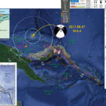
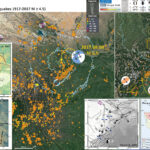
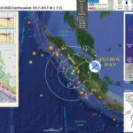
We just had an earthquake in the Mentawai region of the Sunda subduction zone offshore of Sumatra. Here is the USGS website for this M 6.3 earthquake.
Based upon the hypocentral depth and the current estimate of the location of the subduction zone fault, this appears to be a subduction zone interface earthquake.
This M 6.3 earthquake happened near the location of an M 7.6 earthquake on 2009.09.30. Here is the USGS website for this M 7.6 earthquake. The M 7.6 earthquake was deep in the downgoing slab (oceanic crust of the India-Australia plate).
There was an M 6.4 earthquake further to the south on 2017.08.13 and here is my report for that earthquake. These two earthquakes are probably not related.
Today’s earthquake happened in a region of the subduction zone that has not yet ruptured in recent times (with a large magnitude earthquake). The city of Padang, due East of this earthquake, is low lying with millions of people living and working at elevations of less than a few meters. The residents of Padang have a high exposure to earthquake and tsunami risk associated with this subduction zone. Today’s earthquake also happened in a region of the subduction zone that may have a lower amount of seismic coupling (i.e. a lower amount of “stick” on the fault). See the Chlieh et al. (2008) figures in this report and poster.

Below is my interpretive poster for this earthquake

I plot the seismicity from the past month, with color representing depth and diameter representing magnitude (see legend). I also include USGS epicenters from 1917-2017 for magnitudes M ≥ 7.5.

  • I placed a moment tensor / focal mechanism legend on the poster. There is more material from the USGS web sites about moment tensors and focal mechanisms (the beach ball symbols). Both moment tensors and focal mechanisms are solutions to seismologic data that reveal two possible interpretations for fault orientation and sense of motion. One must use other information, like the regional tectonics, to interpret which of the two possibilities is more likely.
  • I also include the shaking intensity contours on the map. These use the Modified Mercalli Intensity Scale (MMI; see the legend on the map). This is based upon a computer model estimate of ground motions, different from the “Did You Feel It?” estimate of ground motions that is actually based on real observations. The MMI is a qualitative measure of shaking intensity. More on the MMI scale can be found here and here. This is based upon a computer model estimate of ground motions, different from the “Did You Feel It?” estimate of ground motions that is actually based on real observations.
  • I include the slab contours plotted (Hayes et al., 2012), which are contours that represent the depth to the subduction zone fault. These are mostly based upon seismicity. The depths of the earthquakes have considerable error and do not all occur along the subduction zone faults, so these slab contours are simply the best estimate for the location of the fault.

    I include some inset figures in the poster.

  • In the upper left corner, I include a map from Hayes et al. (2013) that shows the epicenters of earthquakes from the past century or so. There is also a cross section that is in the region of the 2007 and 2017 M 8.4 and M 6.4 earthquakes. I also placed a C-C’ green line on the main map to show where this cross section is compared to the other features on my map. I placed a blue star in the general location of the M 6.4 earthquake.
  • In the upper right corner, I include a map I made that delineates the spatial extent for historic earthquakes along the Sunda Megathrust. This came from a paper that I had submitted to Marine Geology. I include this figure below with attributions to the publications that I used as references for this map.
  • In the lower right corner, I present a figure from Chlieh et al. (2008 ). These authors use GPS and coral geodetic and paleogeodetic data to constrain the proportion of the plate motion rates that are accumulated as tectonic strain along the megathrust fault. Basically, this means how much % that the fault is storing energy to be released in subduction zone earthquakes. This is just a model and is limited by the temporal and spatial extent of their observations which form the basis for their model. However, this is a well respected approach to estimate the potential for future earthquake (given the assumptions that I here mention).


  • Here is the interpretive poster for the M 6.4 earthquake from 2017.08.13.

  • Here is my map. I include the references below in blockquote.

  • Sumatra core location and plate setting map with sedimentary and erosive systems figure. A. India-Australia plate subducts northeastwardly beneath the Sunda plate (part of Eurasia) at modern rates (GPS velocities are based on regional modeling of Bock et al, 2003 as plotted in Subarya et al., 2006). Historic earthquake ruptures (Bilham, 2005; Malik et al., 2011) are plotted in orange. 2004 earthquake and 2005 earthquake 5 meter slip contours are plotted in orange and green respectively (Chlieh et al., 2007, 2008). Bengal and Nicobar fans cover structures of the India-Australia plate in the northern part of the map. RR0705 cores are plotted as light blue. SRTM bathymetry and topography is in shaded relief and colored vs. depth/elevation (Smith and Sandwell, 1997). B. Schematic illustration of geomorphic elements of subduction zone trench and slope sedimentary settings. Submarine channels, submarine canyons, dune fields and sediment waves, abyssal plain, trench axis, plunge pool, apron fans, and apron fan channels are labeled here. Modified from Patton et al. (2013 a).

  • This is the main figure from Hayes et al. (2013) from the Seismicity of the Earth series. There is a map with the slab contours and seismicity both colored vs. depth. There are also some cross sections of seismicity plotted, with locations shown on the map.

  • Here is a great figure from Philobosian et al. (2014) that shows the slip patches from the subduction zone earthquakes in this region.

  • Map of Southeast Asia showing recent and selected historical ruptures of the Sunda megathrust. Black lines with sense of motion are major plate-bounding faults, and gray lines are seafloor fracture zones. Motions of Australian and Indian plates relative to Sunda plate are from the MORVEL-1 global model [DeMets et al., 2010]. The fore-arc sliver between the Sunda megathrust and the strike-slip Sumatran Fault becomes the Burma microplate farther north, but this long, thin strip of crust does not necessarily all behave as a rigid block. Sim = Simeulue, Ni = Nias, Bt = Batu Islands, and Eng = Enggano. Brown rectangle centered at 2°S, 99°E delineates the area of Figure 3, highlighting the Mentawai Islands. Figure adapted from Meltzner et al. [2012] with rupture areas and magnitudes from Briggs et al. [2006], Konca et al. [2008], Meltzner et al. [2010], Hill et al. [2012], and references therein.

  • This is a figure from Philobosian et al. (2012) that shows a larger scale view for the slip patches in this region. Note that today’s earthquake happened at the edge of the 7.9 earthquake slip patch.

  • Recent and ancient ruptures along the Mentawai section of the Sunda megathrust. Colored patches are surface projections of 1-m slip contours of the deep megathrust ruptures on 12–13 September 2007 (pink to red) and the shallow rupture on 25 October 2010 (green). Dashed rectangles indicate roughly the sections that ruptured in 1797 and 1833. Ancient ruptures are adapted from Natawidjaja et al. [2006] and recent ones come from Konca et al. [2008] and Hill et al. (submitted manuscript, 2012). Labeled points indicate coral study sites Sikici (SKC), Pasapuat (PSP), Simanganya (SMY), Pulau Pasir (PSR), and Bulasat (BLS).

  • Here are a series of figures from Chlieh et al. (2008 ) that show their data sources and their modeling results. I include their figure captions below in blockquote.
  • This figure shows the coupling model (on the left) and the source data for their inversions (on the right). Their source data are vertical deformation rates as measured along coral microattols. These are from data prior to the 2004 SASZ earthquake.

  • Distribution of coupling on the Sumatra megathrust derived from the formal inversion of the coral and of the GPS data (Tables 2, 3, and 4) prior to the 2004 Sumatra-Andaman earthquake (model I-a in Table 7). (a) Distribution of coupling on the megathrust. Fully coupled areas are red, and fully creeping areas are white. Three strongly coupled patches are revealed beneath Nias island, Siberut island, and Pagai island. The annual moment deficit rate corresponding to that model is 4.0 X 10^20 N m/a. (b) Observed (black vectors) and predicted (red vectors) horizontal velocities appear. Observed and predicted vertical displacements are shown by color-coded large and small circles, respectively. The Xr^2 of this model is 3.9 (Table 7).

  • This is a similar figure, but based upon observations between June 2005 and October 2006.

  • Distribution of coupling on the Sumatra megathrust derived from the formal inversion of the horizontal velocities and uplift rates derived from the CGPS measurements at the SuGAr stations (processed at SOPAC). To reduce the influence of postseismic deformation caused by the March 2005 Nias-Simeulue rupture, velocities were determined for the period between June 2005 and October 2006. (a) Distribution of coupling on the megathrust. Fully coupled areas are red and fully creeping areas are white. This model reveals strong coupling beneath the Mentawai Islands (Siberut, Sipora, and Pagai islands), offshore Padang city, and suggests that the megathrust south of Bengkulu city is creeping at the plate velocity. (b) Comparison of observed (green) and predicted (red) velocities. The Xr^2 associated to that model is 24.5 (Table 8).

  • This is a similar figure, but based on all the data.

  • Distribution of coupling on the Sumatra megathrust derived from the formal inversion of all the data (model J-a, Table 8). (a) Distribution of coupling on the megathrust. Fully coupled areas are red, and fully creeping areas are white. This model shows strong coupling beneath Nias island and beneath the Mentawai (Siberut, Sipora and Pagai) islands. The rate of accumulation of moment deficit is 4.5 X 10^20 N m/a. (b) Comparison of observed (black arrows for pre-2004 Sumatra-Andaman earthquake and green arrows for post-2005 Nias earthquake) and predicted velocities (in red). Observed and predicted vertical displacements are shown by color-coded large and small circles (for the corals) and large and small diamonds (for the CGPS), respectively. The Xr^2 of this model is 12.8.

  • Here is the figure I included in the poster above.

  • Comparison of interseismic coupling along the megathrust with the rupture areas of the great 1797, 1833, and 2005 earthquakes. The southernmost rupture area of the 2004 Sumatra-Andaman earthquake lies north of our study area and is shown only for reference. Epicenters of the 2007 Mw 8.4 and Mw 7.9 earthquakes are also shown for reference. (a) Geometry of the locked fault zone corresponding to forward model F-f (Figure 6c). Below the Batu Islands, where coupling occurs in a narrow band, the largest earthquake for the past 260 years has been a Mw 7.7 in 1935 [Natawidjaja et al., 2004; Rivera et al., 2002]. The wide zones of coupling, beneath Nias, Siberut, and Pagai islands, coincide well with the source of great earthquakes (Mw > 8.5) in 2005 from Konca et al. [2007] and in 1797 and 1833 from Natawidjaja et al. [2006]. The narrow locked patch beneath the Batu islands lies above the subducting fossil Investigator Fracture Zone. (b) Distribution of interseismic coupling corresponding to inverse model J-a (Figure 10). The coincidence of the high coupling area (orange-red dots) with the region of high coseismic slip during the 2005 Nias-Simeulue earthquake suggests that strongly coupled patches during interseismic correspond to seismic asperities during megathrust ruptures. The source regions of the 1797 and 1833 ruptures also correlate well with patches that are highly coupled beneath Siberut, Sipora, and Pagai islands.

  • This figure shows the authors’ estimate for the moment deficit in this region of the subduction zone. This is an estimate of how much the plate convergence rate, that is estimated to accumulate as tectonic strain, will need to be released during subduction zone earthquakes.

  • Latitudinal distributions of seismic moment released by great historical earthquakes and of accumulated deficit of moment due to interseismic locking of the plate interface. Values represent integrals over half a degree of latitude. Accumulated interseismic deficits since 1797, 1833, and 1861 are based on (a) model F-f and (b) model J-a. Seismic moments for the 1797 and 1833 Mentawai earthquakes are estimated based on the work by Natawidjaja et al. [2006], the 2005 Nias-Simeulue earthquake is taken from Konca et al. [2007], and the 2004 Sumatra-Andaman earthquake is taken from Chlieh et al. [2007]. Postseismic moments released in the month that follows the 2004 earthquake and in the 11 months that follows the Nias-Simeulue 2005 earthquake are shown in red and green, respectively, based on the work by Chlieh et al. [2007] and Hsu et al. [2006].

  • For a review of the 2004 and 2005 Sumatra Andaman subduction zone (SASZ) earthquakes, please check out my Earthquake Report here. Below is the poster from that report. On that report page, I also include some information about the 2012 M 8.6 and M 8.2 Wharton Basin earthquakes.
    • I include some inset figures in the poster.
    • In the upper left corner, I include a map that shows the extent of historic earthquakes along the SASZ offshore of Sumatra. This map is a culmination of a variety of papers (summarized and presented in Patton et al., 2015).
    • In the upper right corner I include a figure that is presented by Chlieh et al. (2007). These figures show model results from several models. Each model is represented by a map showing the amount that the fault slipped in particular regions. I present this figure below.
    • In the lower right corner I present a figure from Prawirodirdjo et al. (2010). This figure shows the coseismic vertical and horizontal motions from the 2004 and 2005 earthquakes as measured at GPS sites.
    • In the lower left corner are the MMI intensity maps for the two SASZ earthquakes. Note these are at different map scales. I also include the MMI attenuation curves for these earthquakes below the maps. These plots show the reported MMI intensity data as they relate to two plots of modeled estimates (the orange and green lines). These green dots are from the USGS “Did You Feel It?” reports compared to the estimates of ground shaking from Ground Motion Prediction Equation (GMPE) estimates. GMPE are empirical relations between earthquakes and recorded seismologic observations from those earthquakes, largely controlled by distance to the fault, ray path (direction and material properties), and site effects (the local geology). When seismic waves propagate through sediment, the magnitude of the ground motions increases in comparison to when seismic waves propagate through bedrock. The orange line is a regression of data for the central and eastern US and the green line is a regression through data from the western US.


  • The 2004/2005 SASZ earthquakes also tended to load strain in the crust in different locations. On 2012.04.11 there was a series of strike-slip earthquakes in the India plate crust to the west of the 2004/2005 earthquakes. The two largest magnitudes for these earthquakes were M 8.6 and M 8.2. The M 8.6 is the largest strike-slip earthquake ever recorded.
  • On 2016.03.22 there was another large strike-slip earthquake in the India-Australia plate. This is probably related to this entire suite of subduction zone and intraplate earthquakes. I presented an interpretive poster about this M 7.8 earthquake here. Below is my interpretive poster for the M 7.8 earthquake. Here is the USGS website for this earthquake.
  • I include a map in the upper right corner that shows the historic earthquake rupture areas.

  • Here is a poster that shows some earthquakes in the Andaman Sea. This is from my earthquake report from 2015.11.08.

  • This map shows the fracture zones in the India-Australia plate.

References:

  • Abercrombie, R.E., Antolik, M., Ekstrom, G., 2003. The June 2000 Mw 7.9 earthquakes south of Sumatra: Deformation in the India–Australia Plate. Journal of Geophysical Research 108, 16.
  • Bassin, C., Laske, G. and Masters, G., The Current Limits of Resolution for Surface Wave Tomography in North America, EOS Trans AGU, 81, F897, 2000.
  • Bock, Y., Prawirodirdjo, L., Genrich, J.F., Stevens, C.W., McCaffrey, R., Subarya, C., Puntodewo, S.S.O., Calais, E., 2003. Crustal motion in Indonesia from Global Positioning System measurements: Journal of Geophysical Research, v. 108, no. B8, 2367, doi: 10.1029/2001JB000324.
  • Bothara, J., Beetham, R.D., Brunston, D., Stannard, M., Brown, R., Hyland, C., Lewis, W., Miller, S., Sanders, R., Sulistio, Y., 2010. General observations of effects of the 30th September 2009 Padang earthquake, Indonesia. Bulletin of the New Zealand Society for Earthquake Engineering 43, 143-173.
  • Chlieh, M., Avouac, J.-P., Hjorleifsdottir, V., Song, T.-R.A., Ji, C., Sieh, K., Sladen, A., Hebert, H., Prawirodirdjo, L., Bock, Y., Galetzka, J., 2007. Coseismic Slip and Afterslip of the Great (Mw 9.15) Sumatra-Andaman Earthquake of 2004. Bulletin of the Seismological Society of America 97, S152-S173.
  • Chlieh, M., Avouac, J.P., Sieh, K., Natawidjaja, D.H., Galetzka, J., 2008. Heterogeneous coupling of the Sumatran megathrust constrained by geodetic and paleogeodetic measurements: Journal of Geophysical Research, v. 113, B05305, doi: 10.1029/2007JB004981.
  • DEPLUS, C. et al., 1998 – Direct evidence of active derormation in the eastern Indian oceanic plate, Geology.
  • DYMENT, J., CANDE, S.C. & SINGH, S., 2007 – Oceanic lithosphere subducting beneath the Sunda Trench: the Wharton Basin revisited. European Geosciences Union General Assembly, Vienna, 15-20/05.
  • Hayes, G. P., Wald, D. J., and Johnson, R. L., 2012. Slab1.0: A three-dimensional model of global subduction zone geometries in J. Geophys. Res., 117, B01302, doi:10.1029/2011JB008524.
  • Hayes, G.P., Bernardino, Melissa, Dannemann, Fransiska, Smoczyk, Gregory, Briggs, Richard, Benz, H.M., Furlong, K.P., and Villaseñor, Antonio, 2013. Seismicity of the Earth 1900–2012 Sumatra and vicinity: U.S. Geological Survey Open-File Report 2010–1083-L, scale 1:6,000,000, https://pubs.usgs.gov/of/2010/1083/l/.
  • JACOB, J., DYMENT, J., YATHEESH, V. & BHATTACHARYA, G.C., 2009 – Marine magnetic anomalies in the NE Indian Ocean: the Wharton and Central Indian basins revisited. European Geosciences Union General Assembly, Vienna, 19-24/04.
  • Ji, C., D.J. Wald, and D.V. Helmberger, Source description of the 1999 Hector Mine, California earthquake; Part I: Wavelet domain inversion theory and resolution analysis, Bull. Seism. Soc. Am., Vol 92, No. 4. pp. 1192-1207, 2002.
  • Ishii, M., Shearer, P.M., Houston, H., Vidale, J.E., 2005. Extent, duration and speed of the 2004 Sumatra-Andaman earthquake imaged by the Hi-Net array. Nature 435, 933.
  • Kanamori, H., Rivera, L., Lee, W.H.K., 2010. Historical seismograms for unravelling a mysterious earthquake: The 1907 Sumatra Earthquake. Geophysical Journal International 183, 358-374.
  • Konca, A.O., Avouac, J., Sladen, A., Meltzner, A.J., Sieh, K., Fang, P., Li, Z., Galetzka, J., Genrich, J., Chlieh, M., Natawidjaja, D.H., Bock, Y., Fielding, E.J., Ji, C., Helmberger, D., 2008. Partial Rupture of a Locked Patch of the Sumatra Megathrust During the 2007 Earthquake Sequence. Nature 456, 631-635.
  • Maus, S., et al., 2009. EMAG2: A 2–arc min resolution Earth Magnetic Anomaly Grid compiled from satellite, airborne, and marine magnetic measurements, Geochem. Geophys. Geosyst., 10, Q08005, doi:10.1029/2009GC002471.
  • Malik, J.N., Shishikura, M., Echigo, T., Ikeda, Y., Satake, K., Kayanne, H., Sawai, Y., Murty, C.V.R., Dikshit, D., 2011. Geologic evidence for two pre-2004 earthquakes during recent centuries near Port Blair, South Andaman Island, India: Geology, v. 39, p. 559-562.
  • Meltzner, A.J., Sieh, K., Chiang, H., Shen, C., Suwargadi, B.W., Natawidjaja, D.H., Philobosian, B., Briggs, R.W., Galetzka, J., 2010. Coral evidence for earthquake recurrence and an A.D. 1390–1455 cluster at the south end of the 2004 Aceh–Andaman rupture. Journal of Geophysical Research 115, 1-46.
  • Meng, L., Ampuero, J.-P., Stock, J., Duputel, Z., Luo, Y., and Tsai, V.C., 2012. Earthquake in a Maze: Compressional Rupture Branching During the 2012 Mw 8.6 Sumatra Earthquake in Science, v. 337, p. 724-726.
  • Natawidjaja, D.H., Sieh, K., Chlieh, M., Galetzka, J., Suwargadi, B., Cheng, H., Edwards, R.L., Avouac, J., Ward, S.N., 2006. Source parameters of the great Sumatran megathrust earthquakes of 1797 and 1833 inferred from coral microatolls. Journal of Geophysical Research 111, 37.
  • Newcomb, K.R., McCann, W.R., 1987. Seismic History and Seismotectonics of the Sunda Arc. Journal of Geophysical Research 92, 421-439.
  • Philibosian, B., Sieh, K., Natawidjaja, D.H., Chiang, H., Shen, C., Suwargadi, B., Hill, E.M., Edwards, R.L., 2012. An ancient shallow slip event on the Mentawai segment of the Sunda megathrust, Sumatra. Journal of Geophysical Research 117, 12.
  • Prawirodirdjo, P., McCaffrey,R., Chadwell, D., Bock, Y, and Subarya, C., 2010. Geodetic observations of an earthquake cycle at the Sumatra subduction zone: Role of interseismic strain segmentation, JOURNAL OF GEOPHYSICAL RESEARCH, v. 115, B03414, doi:10.1029/2008JB006139
  • Rivera, L., Sieh, K., Helmberger, D., Natawidjaja, D.H., 2002. A Comparative Study of the Sumatran Subduction-Zone Earthquakes of 1935 and 1984. BSSA 92, 1721-1736.
  • Shearer, P., and Burgmann, R., 2010. Lessons Learned from the 2004 Sumatra-Andaman Megathrust Rupture, Annu. Rev. Earth Planet. Sci. v. 38, pp. 103–31
  • SATISH C. S, CARTON H, CHAUHAN A.S., et al., 2011 – Extremely thin crust in the Indian Ocean possibly resulting from Plume-Ridge Interaction, Geophysical Journal International.
  • Sieh, K., Natawidjaja, D.H., Meltzner, A.J., Shen, C., Cheng, H., Li, K., Suwargadi, B.W., Galetzka, J., Philobosian, B., Edwards, R.L., 2008. Earthquake Supercycles Inferred from Sea-Level Changes Recorded in the Corals of West Sumatra. Science 322, 1674-1678.
  • Singh, S.C., Carton, H.L., Tapponnier, P, Hananto, N.D., Chauhan, A.P.S., Hartoyo, D., Bayly, M., Moeljopranoto, S., Bunting, T., Christie, P., Lubis, H., and Martin, J., 2008. Seismic evidence for broken oceanic crust in the 2004 Sumatra earthquake epicentral region, Nature Geoscience, v. 1, pp. 5.
  • Smith, W.H.F., Sandwell, D.T., 1997. Global seafloor topography from satellite altimetry and ship depth soundings: Science, v. 277, p. 1,957-1,962.
  • Sorensen, M.B., Atakan, K., Pulido, N., 2007. Simulated Strong Ground Motions for the Great M 9.3 Sumatra–Andaman Earthquake of 26 December 2004. BSSA 97, S139-S151.
  • Subarya, C., Chlieh, M., Prawirodirdjo, L., Avouac, J., Bock, Y., Sieh, K., Meltzner, A.J., Natawidjaja, D.H., McCaffrey, R., 2006. Plate-boundary deformation associated with the great Sumatra–Andaman earthquake: Nature, v. 440, p. 46-51.
  • Tolstoy, M., Bohnenstiehl, D.R., 2006. Hydroacoustic contributions to understanding the December 26th 2004 great Sumatra–Andaman Earthquake. Survey of Geophysics 27, 633-646.
  • Zhu, Lupei, and Donald V. Helmberger. “Advancement in source estimation techniques using broadband regional seismograms.” Bulletin of the Seismological Society of America 86.5 (1996): 1634-1641.

#Earthquake Report: North Bismarck plate

Well, what have we here? We have an interesting crustal earthquake in the North Bismarck plate. Why is it interesting? This is an interesting earthquake because of its orientation and mechanism.
This region of the world is one of the most tectonically active areas, where plate convergence, spreading ridges, and transform faults all interplay in a complicated manner. Though, typically, most earthquakes easily fit into the tectonic models that have been developed to date. Today’s earthquake does not readily fit into any fault map that I have found (but please let me know if this is incorrect!).
The majority of the seismicity in this region is due to the compressional tectonics of subduction zones that form the New Britain trench, the San Christobal trench, and the South Solomon trench. I have presented a number of #EarthquakeReports for these subduction zones (see a list of them at the bottom of this page, above the references). The New Britain (NB) and San Christobal (SC) tectonic domains have earthquakes with compressional moment tensors oriented perpendicular to the trench, and are separated by a small domain that has strike-slip moment tensors. I summarize these different domains in a poster below.
The major strike-slip fault that separates these convergent domains is connect to a series of enechelon oceanic spreading centers (mid ocean ridges) that form the N. and S. Bismarck plates. This left-lateral strike-slip fault is currently mapped to terminate at the spreading ridge. When I first saw the earthquake on the USGS feed (here is the USGS website for this earthquake), I thought it might be an extension of this left-lateral strike-slip fault. The USGS has not generated a moment tensor, but the geoscope page from IPGP (here) has a focal mechanism from SCARDEC that shows a strike-slip fault plane solution. Without looking at the details, I thought, “yup, strike-slip, as I thought it would be.” But, upon ruminating on this, I realized that it is the opposite sense of motion to be along an extension of this left-lateral strike-slip fault! If the earthquake is oriented on the northwest striking solution, then it would be a right-lateral strike-slip earthquake. So, I remain befuddled as to which fault plane solution is correct.

Below is my interpretive poster for this earthquake.

I plot the seismicity from the past year, with color representing depth and diameter representing magnitude (see legend).

  • I placed a moment tensor / focal mechanism legend on the poster. There is more material from the USGS web sites about moment tensors and focal mechanisms (the beach ball symbols). Both moment tensors and focal mechanisms are solutions to seismologic data that reveal two possible interpretations for fault orientation and sense of motion. One must use other information, like the regional tectonics, to interpret which of the two possibilities is more likely. The moment tensor shows northeast-southwest compression, perpendicular to the convergence at these plate boundaries.
  • I also include the shaking intensity contours on the map. These use the Modified Mercalli Intensity Scale (MMI; see the legend on the map). This is based upon a computer model estimate of ground motions, different from the “Did You Feel It?” estimate of ground motions that is actually based on real observations. The MMI is a qualitative measure of shaking intensity. More on the MMI scale can be found here and here. This is based upon a computer model estimate of ground motions, different from the “Did You Feel It?” estimate of ground motions that is actually based on real observations.
  • I include the slab contours plotted (Hayes et al., 2012), which are contours that represent the depth to the subduction zone fault. These are mostly based upon seismicity. The depths of the earthquakes have considerable error and do not all occur along the subduction zone faults, so these slab contours are simply the best estimate for the location of the fault.
  • I include some inset figures.

  • In the upper left corner a figure from Oregon State University, which are based upon Hamilton (1979). “Tectonic microplates of the Melanesian region. Arrows show net plate motion relative to the Australian Plate.” This is from Johnson, 1976. To the right of the map is a cross section, showing how the Solomon Sea plate subducts beneath the S. Bismarck plate.
  • In the lower left corner is a more detailed map of the plate boundary faults in this region. I place a blue star in the general location of today’s M 6.4 earthquake (also placed on other inset figures).
  • In the upper right corner is a figure from Baldwin et al. (2012). This figure shows a series of cross sections along this convergent plate boundary from the Solomon Islands in the east to Papua New Guinea in the west. Cross sections ‘C’ and ‘D’ are the most representative for the earthquakes today. Note that today’s earthquake is not aligned with any plate boundary faults. I present the map and this figure again below, with their original captions.
  • In the lower right corner is a generalized tectonic map of the region from Holm et al., 2016. This map shows the major plate boundary faults. Active subduction zones have shaded triangle fault symbols, while inactive subduction zones have un-shaded triangle fault line symbols.


  • In earlier earthquake reports, I discussed seismicity from 2000-2015 here. The seismicity on the west of this region appears aligned with north-south shortening along the New Britain trench, while seismicity on the east of this region appears aligned with more east-west shortening. Here is a map that I put together where I show these two tectonic domains with the seismicity from this time period (today’s earthquakes are not plotted on this map, but one may see where they might plot).


Background Figures

  • This figure shows an interpretation of the regional tectonics (Holm et al., 2016). I include the figure caption below as a blockquote.

  • Tectonic setting of Papua New Guinea and Solomon Islands. a) Regional plate boundaries and tectonic elements. Light grey shading illustrates bathymetry b 2000 m below sea level indicative of continental or arc crust, and oceanic plateaus; 1000 m depth contour is also shown. Adelbert Terrane (AT); Bismarck Sea fault (BSF); Bundi fault zone (BFZ); Feni Deep (FD); Finisterre Terrane (FT); Gazelle Peninsula (GP); Kia-Kaipito-Korigole fault zone (KKKF); Lagaip fault zone (LFZ); Mamberamo thrust belt (MTB); Manus Island (MI); New Britain (NB); New Ireland (NI); North Sepik arc (NSA); Ramu-Markham fault (RMF); Weitin Fault (WF);West Bismarck fault (WBF); Willaumez-Manus Rise (WMR).

  • This figure shows details of the regional tectonics (Holm et al., 2016). I include the figure caption below as a blockquote.

  • a) Present day tectonic features of the Papua New Guinea and Solomon Islands region as shown in plate reconstructions. Sea floor magnetic anomalies are shown for the Caroline plate (Gaina and Müller, 2007), Solomon Sea plate (Gaina and Müller, 2007) and Coral Sea (Weissel and Watts, 1979). Outline of the reconstructed Solomon Sea slab (SSP) and Vanuatu slab (VS)models are as indicated. b) Cross-sections related to the present day tectonic setting. Section locations are as indicated. Bismarck Sea fault (BSF); Feni Deep (FD); Louisiade Plateau
    (LP); Manus Basin (MB); New Britain trench (NBT); North Bismarck microplate (NBP); North Solomon trench (NST); Ontong Java Plateau (OJP); Ramu-Markham fault (RMF); San Cristobal trench (SCT); Solomon Sea plate (SSP); South Bismarck microplate (SBP); Trobriand trough (TT); projected Vanuatu slab (VS); West Bismarck fault (WBF); West Torres Plateau (WTP); Woodlark Basin (WB).

  • This map shows plate velocities and euler poles for different blocks. Note the counterclockwise motion of the plate that underlies the Solomon Sea (Baldwin et al., 2012). I include the figure caption below as a blockquote.

  • Tectonic maps of the New Guinea region. (a) Seismicity, volcanoes, and plate motion vectors. Plate motion vectors relative to the Australian plate are surface velocity models based on GPS data, fault slip rates, and earthquake focal mechanisms (UNAVCO, http://jules.unavco.org/Voyager/Earth). Earthquake data are sourced from the International Seismological Center EHB Bulletin (http://www.isc.ac.uk); data represent events from January 1994 through January 2009 with constrained focal depths. Background image is generated from http://www.geomapapp.org. Abbreviations: AB, Arafura Basin; AT, Aure Trough; AyT, Ayu Trough; BA, Banda arc; BSSL, Bismarck Sea seismic lineation; BH, Bird’s Head; BT, Banda Trench; BTFZ, Bewani-Torricelli fault zone; DD, Dayman Dome; DEI, D’Entrecasteaux Islands; FP, Fly Platform; GOP, Gulf of Papua; HP, Huon peninsula; LA, Louisiade Archipelago; LFZ, Lowlands fault zone; MaT, Manus Trench; ML, Mt. Lamington; MT, Mt. Trafalgar; MuT, Mussau Trough; MV, Mt. Victory; MTB, Mamberamo thrust belt; MVF, Managalase Plateau volcanic field; NBT, New Britain Trench; NBA, New Britain arc; NF, Nubara fault; NGT, New Guinea Trench; OJP, Ontong Java Plateau; OSF, Owen Stanley fault zone; PFTB, Papuan fold-and-thrust belt; PP, Papuan peninsula; PRi, Pocklington Rise; PT, Pocklington Trough; RMF, Ramu-Markham fault; SST, South Solomons Trench; SA, Solomon arc; SFZ, Sorong fault zone; ST, Seram Trench; TFZ, Tarera-Aiduna fault zone; TJ, AUS-WDKPAC triple junction; TL, Tasman line; TT, Trobriand Trough;WD, Weber Deep;WB, Woodlark Basin;WFTB, Western (Irian) fold-and-thrust belt; WR,Woodlark Rift; WRi, Woodlark Rise; WTB, Weyland thrust; YFZ, Yapen fault zone.White box indicates the location shown in Figure 3. (b) Map of plates, microplates, and tectonic blocks and elements of the New Guinea region. Tectonic elements modified after Hill & Hall (2003). Abbreviations: ADB, Adelbert block; AOB, April ultramafics; AUS, Australian plate; BHB, Bird’s Head block; CM, Cyclops Mountains; CWB, Cendrawasih block; CAR, Caroline microplate; EMD, Ertsberg Mining District; FA, Finisterre arc; IOB, Irian ophiolite belt; KBB, Kubor & Bena blocks (including Bena Bena terrane); LFTB, Lengguru fold-and-thrust belt; MA, Mapenduma anticline; MB, Mamberamo Basin block; MO, Marum ophiolite belt; MHS, Manus hotspot; NBS, North Bismarck plate; NGH, New Guinea highlands block; NNG, Northern New Guinea block; OKT, Ok Tedi mining district; PAC, Pacific plate; PIC, Porgera intrusive complex; PSP, Philippine Sea plate; PUB, Papuan Ultramafic Belt ophiolite; SB, Sepik Basin block; SDB, Sunda block; SBS, South Bismarck plate; SIB, Solomon Islands block; WP, Wandamen peninsula; WDK, Woodlark microplate; YQ, Yeleme quarries.

  • This figure incorporates cross sections and map views of various parts of the regional tectonics (Baldwin et al., 2012). The New Britain region is in the map near the A and B sections. I include the figure caption below as a blockquote.

  • Oblique block diagram of New Guinea from the northeast with schematic cross sections showing the present-day plate tectonic setting. Digital elevation model was generated from http://www.geomapapp.org. Oceanic crust in tectonic cross sections is shown by thick black-and-white hatched lines, with arrows indicating active subduction; thick gray-and-white hatched lines indicate uncertain former subduction. Continental crust, transitional continental crust, and arc-related crust are shown without pattern. Representative geologic cross sections across parts of slices C and D are marked with transparent red ovals and within slices B and E are shown by dotted lines. (i ) Cross section of the Papuan peninsula and D’Entrecasteaux Islands modified from Little et al. (2011), showing the obducted ophiolite belt due to collision of the Australian (AUS) plate with an arc in the Paleogene, with later Pliocene extension and exhumation to form the D’Entrecasteaux Islands. (ii ) Cross section of the Papuan peninsula after Davies & Jaques (1984) shows the Papuan ophiolite thrust over metamorphic rocks of AUS margin affinity. (iii ) Across the Papuan mainland, the cross section after Crowhurst et al. (1996) shows the obducted Marum ophiolite and complex folding and thrusting due to collision of the Melanesian arc (the Adelbert, Finisterre, and Huon blocks) in the Late Miocene to recent. (iv) Across the Bird’s Head, the cross section after Bailly et al. (2009) illustrates deformation in the Lengguru fold-and-thrust belt as a result of Late Miocene–Early Pliocene northeast-southwest shortening, followed by Late Pliocene–Quaternary extension. Abbreviations as in Figure 2, in addition to NI, New Ireland; SI, Solomon Islands; SS, Solomon Sea; (U)HP, (ultra)high-pressure.


Background Videos

  • I put together an animation that shows the seismicity for this region from 1900-2016 for earthquakes with magnitude of M ≥ 6.5. Here is the USGS query I used to search for these data used in this animation. I show the location of the Benz et al. (2011) cross section E-E’ as a yellow line on the main map.
  • In this animation, I include some figures from the interpretive poster above. I also include a tectonic map based upon Hamilton (1979). Music is from copyright free music online and is entitled “Sub Strut.” Above the video I present a map showing all the earthquakes presented in the video.
  • Here is a link to the embedded video below (5 MB mp4)


References:

Earthquake Report: Mid Atlantic Ridge (Chain fracture zone)

If there was an earthquake in the middle of the ocean, and nobody felt it… would it still be an earthquake? Maybe we need to get the Karl Popper out for a good read…
There was a good sized shaker less than an hour ago (at the time I started writing this, when it was first estimated to be M 6.8). Here is the USGS website for the M 6.6 earthquake that appears to be associated with the Chan fracture zone.
This may be related to a recent earthquake on the Romanche fracture zone, but it is probably too far away. Here is my report for this M 7.1 earthquake from 2016.08.29.

Below is my interpretive poster for this earthquake

I plot the seismicity from the past month, with color representing depth and diameter representing magnitude (see legend). I also include USGS epicenters from 1900-2016 for magnitudes M ≥ 6.0.
I also include the USGS moment tensor for today’s earthquake.

  • I placed a moment tensor / focal mechanism legend on the poster. There is more material from the USGS web sites about moment tensors and focal mechanisms (the beach ball symbols). Both moment tensors and focal mechanisms are solutions to seismologic data that reveal two possible interpretations for fault orientation and sense of motion. One must use other information, like the regional tectonics, to interpret which of the two possibilities is more likely. Based upon the series of earthquakes and the mapped faults, I interpret this M 5.1 earthquake as a left-lateral strike-slip earthquake related to slip associated with the Gorda plate.
  • I also include the shaking intensity contours on the map. These use the Modified Mercalli Intensity Scale (MMI; see the legend on the map). This is based upon a computer model estimate of ground motions, different from the “Did You Feel It?” estimate of ground motions that is actually based on real observations. The MMI is a qualitative measure of shaking intensity. More on the MMI scale can be found here and here. This is based upon a computer model estimate of ground motions, different from the “Did You Feel It?” estimate of ground motions that is actually based on real observations.

    I include some inset figures in the poster.

  • In the upper left corner is a map that shows the age of the oceanic crust in Million Years B.P. (before present). The MAR is highlighted because it is of about zero age, so is shown as red (Müller et al., 2008). I place a blue star in the general location of this M 6.6 earthquake (as for the other inset maps).
  • In the lower left corner is a map that shows a revised interpretation of the timing and orientations of the initial breakup and formation of the MAR and the Atlantic Ocean from Torsvik et al. (2009)
  • In the lower right corner is a diagram that illustrates how Earth’s magnetic field reversals are recorded in the oceanic crust through time. This is one of the principal evidences that supports the hypotheses regarding plate tectonics. From top to bottom (earlier in time to later in time, where t = some time).
    • t = 0 Earth’s magnetic field is the same as it is today. We term this “normal” polarization. Rocks (and sediments) formed at this time can have magnetic minerals and grains align with the magnetic field orientation at that time.
      Colored oceanic crust (in this diagram) represents crust formed when the magnetic field is oriented like it is today.
    • t = 1 Tens of thousands to hundreds of thousands years later, as the plates diverge from the spreading ridge, decompression melting leads to accretion of new oceanic crust at the ridge. At this time, the magnetic field has reversed (north pole becomes south pole, dogs and cats living together (from movie “Ghostbusters”)), so the oceanic crust rock is magnetized with a field oriented opposite from the way it is today. We term this crust to have “reverse” polarization. Then, the magnetic field flips orientation again, becoming normal again. The diagram shows at this time, the crust forming at the ridge is normally polarized.
    • t = 2 Tens of thousands to hundreds of thousands years later, the plates continue to diverge from the spreading ridge forming new crust, and there are additional cycles of flipping magnetic fields. The result is a pattern, symmetrical about the spreading ridge, of oceanic crust that has alternating bands of crust with different polarities.
  • In the upper center is a map that shows the two fracture zones in this region (Romanche and Chain) along with focal mechanisms for earthquakes along these fracture zones. The fracture zones, which offset the Mid Atlantic Ridge (MAR), are transform plate boundaries. Considering the orientation of these fracture zones and the MAR, these earthquakes are right-lateral strike-slip earthquakes. Today’s M 6.6 earthquake is no different. Note how this earthquake is nearly perfect strike slip.
  • In the upper right corner is a larger scale map that shows the details of the sea floor in this region.The majority of the seismicity occurs along the fracture zones, which offset the MAR. Today’s earthquake is most likely associated with strike-slip faulting along the Chan fracture zone.


  • Here is the Bonatti et al. (2001) figure from the interpretive poster above. I include the figure caption as a blockquote below.

  • A: Multibeam topography of Romanche region, showing north-south profiles where sampling was carried out. Black dots and red numbers indicate estimated age (in million years) of lithosphere south of Romanche Transform, assuming spreading half-rate of 17 mm/yr within present-day ridge and transform geometry. White dots indicate epicenters of teleseismically recorded 1970–1995 events (magnitude . 4). FZ is fracture zone. B: Topography and petrology at eastern intersection of Romanche Fracture Zone with Mid-Atlantic Ridge. Data were obtained during expeditions S-16, S-19, and G-96 (Bonatti et al., 1994, 1996). C: Location of A along Mid-Atlantic Ridge.

  • Here is the Müller et al. (2008) figure from the interpretive poster above.

  • Here is the Torsvik et al. (2009) figure from the interpretive poster above. I include the figure caption as a blockquote below.

  • General structural map of the South Atlantic Ocean draped on topographic/bathymetric map from GTOPO 30. Boundaries between the four segments (Equatorial, Central, South and Falkland) are shown by dotted lines (RFZ, Romanche Fracture Zone; FFZ, Florianopolis Fracture Zone; AFFZ, Agulhas– Falkland Fracture Zone). Aptian salt basins (orange), LIPs (P, Parana; E, Etendeka; Karroo, Sierra Leone Rise and Agulhas), Seaward Dipping Reflectors (SDRs, white) and active hotspots (F, Fernando; C, Cameroon; Tr, Trinidade; Sh, St Helena; T, Tristan; V, Vema; B, Bouvet (Meteor) are also shown. Of these hotspots, only Tristan (responsible for the Parana-Etendeka LIP and Rio Grande Rise–Walvis Ridge) is classically considered as a deep plume in the literature (see Torsvik et al. 2006). However, Bouvet (Meteor) possibly responsible for Agulhas, and Maud Rise (East Antarctica) and Madagascar Ridge volcanism could possibly also have a deep plume origin (Section 6). PG, Ponta Grossa Dyke System; PA, Paraguay Dyke system; FI, Falkland Islands.

    References:

  • Abercrombie, R.E. and Ekstrom, G., 2001. Earthquake slip on oceanic transform faults in Nature, v. 410, p. 74-77
  • Bonatti, E., Brunelli, D., Fabretti, P., Ligi, M., Portaro, R.A., and Seyler, M., 2001. Steady-state creation of crust-free lithosphere at cold spots in mid-ocean ridges in Geology, v. 29, no. 11, p. 979-982.
  • Müller, R.D., Sdrolias, M., Gaina, C., and Roest, W.R., 2008. Age, spreading rates and spreading symmetry of the world’s ocean crust in Geochem. Geophys. Geosyst., 9, Q04006, doi:10.1029/2007GC001743
  • Torsvik, T.H., Tousse, S., Labaila, C., and Smethurst, M.A., 2009. A new scheme for the opening of the South Atlantic Ocean and the dissection of an Aptian salt basin in Geophysical Journal INternational, v. 177, p. 1315-1333.

Earthquake Report: Bengkulu (Sumatra)!

Last night (my time) while I was tending to other business, there was an earthquake along the Sunda Megathrust. Here is the USGS website for this M 6.4 earthquake.
This M 6.4 earthquake happened down-dip (“deeper than”) along the megathrust from the 2007.09.12 M 8.4 megathrust earthquake. Here is the USGS website for the M 8.4 earthquake. This M 6.4 earthquake occurred in a region of low seismogenic coupling (as inferred by Chlieh at al., 2008), albeit with sparse GPS data in this region. Chlieh et al. (2008) used coral geodetic and paleogeodetic data, along with Global Positioning System (GPS) observations, to constrain their model. Because there are no forearc islands in this part of the subduction zone, there are no GPS nor coral data with which to constrain their model (so it may underestimate the coupling %, i.e. coupling ratio).
Based upon the USGS fault plane slip model, this M 6.4 earthquake actually happened in a region of higher slip from the M 8.4 earthquake. We may consider this M 6.4 earthquake to be an aftershock of the M 8.4 earthquake.
Here is a report from earthquake-report.com.

Below is my interpretive poster for this earthquake

I plot the seismicity from the past month, with color representing depth and diameter representing magnitude (see legend). I also include USGS epicenters from 1917-2017 for magnitudes M ≥ 7.
I also include the USGS moment tensor for today’s earthquake, as well as for the 2007 M 8.4 earthquake. I label the other epicenters with large magnitudes (2004, 2005, and 2012). Find more details about these earthquakes in my reports listed at the bottom of this page, above the references.

  • I placed a moment tensor / focal mechanism legend on the poster. There is more material from the USGS web sites about moment tensors and focal mechanisms (the beach ball symbols). Both moment tensors and focal mechanisms are solutions to seismologic data that reveal two possible interpretations for fault orientation and sense of motion. One must use other information, like the regional tectonics, to interpret which of the two possibilities is more likely.
  • I also include the shaking intensity contours on the map. These use the Modified Mercalli Intensity Scale (MMI; see the legend on the map). This is based upon a computer model estimate of ground motions, different from the “Did You Feel It?” estimate of ground motions that is actually based on real observations. The MMI is a qualitative measure of shaking intensity. More on the MMI scale can be found here and here. This is based upon a computer model estimate of ground motions, different from the “Did You Feel It?” estimate of ground motions that is actually based on real observations.
  • I include the slab contours plotted (Hayes et al., 2012), which are contours that represent the depth to the subduction zone fault. These are mostly based upon seismicity. The depths of the earthquakes have considerable error and do not all occur along the subduction zone faults, so these slab contours are simply the best estimate for the location of the fault.

    I include some inset figures in the poster.

  • In the upper right corner, I include a map from Hayes et al. (2013) that shows the epicenters of earthquakes from the past century or so. There is also a cross section that is in the region of the 2007 and 2017 M 8.4 and M 6.4 earthquakes. I also placed a C-C’ green line on the main map to show where this cross section is compared to the other features on my map. I placed a blue star in the general location of the M 6.4 earthquake.
  • In the lower left corner, I include a map I made that delineates the spatial extent for historic earthquakes along the Sunda Megathrust. This came from a paper that I had submitted to Marine Geology. I include this figure below with attributions to the publications that I used as references for this map. I outlined the slip patch for the M 8.4 earthquake in transparent orange.
  • In the upper left corner, I present a figure from Chlieh et al. (2008 ). These authors use GPS and coral geodetic and paleogeodetic data to constrain the proportion of the plate motion rates that are accumulated as tectonic strain along the megathrust fault. Basically, this means how much % that the fault is storing energy to be released in subduction zone earthquakes. This is just a model and is limited by the temporal and spatial extent of their observations which form the basis for their model. However, this is a well respected approach to estimate the potential for future earthquake (given the assumptions that I here mention).


  • I prepared this figure to show the difference in MMI Intensity for these two closely spaced earthquakes. The data here come from the USGS websites listed above.

  • Here is my map. I include the references below in blockquote.

  • Sumatra core location and plate setting map with sedimentary and erosive systems figure. A. India-Australia plate subducts northeastwardly beneath the Sunda plate (part of Eurasia) at modern rates (GPS velocities are based on regional modeling of Bock et al, 2003 as plotted in Subarya et al., 2006). Historic earthquake ruptures (Bilham, 2005; Malik et al., 2011) are plotted in orange. 2004 earthquake and 2005 earthquake 5 meter slip contours are plotted in orange and green respectively (Chlieh et al., 2007, 2008). Bengal and Nicobar fans cover structures of the India-Australia plate in the northern part of the map. RR0705 cores are plotted as light blue. SRTM bathymetry and topography is in shaded relief and colored vs. depth/elevation (Smith and Sandwell, 1997). B. Schematic illustration of geomorphic elements of subduction zone trench and slope sedimentary settings. Submarine channels, submarine canyons, dune fields and sediment waves, abyssal plain, trench axis, plunge pool, apron fans, and apron fan channels are labeled here. Modified from Patton et al. (2013 a).

  • This is the main figure from Hayes et al. (2013) from the Seismicity of the Earth series. There is a map with the slab contours and seismicity both colored vs. depth. There are also some cross sections of seismicity plotted, with locations shown on the map.

  • Here is a great figure from Philobosian et al. (2014) that shows the slip patches from the subduction zone earthquakes in this region.

  • Map of Southeast Asia showing recent and selected historical ruptures of the Sunda megathrust. Black lines with sense of motion are major plate-bounding faults, and gray lines are seafloor fracture zones. Motions of Australian and Indian plates relative to Sunda plate are from the MORVEL-1 global model [DeMets et al., 2010]. The fore-arc sliver between the Sunda megathrust and the strike-slip Sumatran Fault becomes the Burma microplate farther north, but this long, thin strip of crust does not necessarily all behave as a rigid block. Sim = Simeulue, Ni = Nias, Bt = Batu Islands, and Eng = Enggano. Brown rectangle centered at 2°S, 99°E delineates the area of Figure 3, highlighting the Mentawai Islands. Figure adapted from Meltzner et al. [2012] with rupture areas and magnitudes from Briggs et al. [2006], Konca et al. [2008], Meltzner et al. [2010], Hill et al. [2012], and references therein.

  • This is a figure from Philobosian et al. (2012) that shows a larger scale view for the slip patches in this region.

  • Recent and ancient ruptures along the Mentawai section of the Sunda megathrust. Colored patches are surface projections of 1-m slip contours of the deep megathrust ruptures on 12–13 September 2007 (pink to red) and the shallow rupture on 25 October 2010 (green). Dashed rectangles indicate roughly the sections that ruptured in 1797 and 1833. Ancient ruptures are adapted from Natawidjaja et al. [2006] and recent ones come from Konca et al. [2008] and Hill et al. (submitted manuscript, 2012). Labeled points indicate coral study sites Sikici (SKC), Pasapuat (PSP), Simanganya (SMY), Pulau Pasir (PSR), and Bulasat (BLS).

  • Here are a series of figures from Chlieh et al. (2008 ) that show their data sources and their modeling results. I include their figure captions below in blockquote.
  • This figure shows the coupling model (on the left) and the source data for their inversions (on the right). Their source data are vertical deformation rates as measured along coral microattols. These are from data prior to the 2004 SASZ earthquake.

  • Distribution of coupling on the Sumatra megathrust derived from the formal inversion of the coral and of the GPS data (Tables 2, 3, and 4) prior to the 2004 Sumatra-Andaman earthquake (model I-a in Table 7). (a) Distribution of coupling on the megathrust. Fully coupled areas are red, and fully creeping areas are white. Three strongly coupled patches are revealed beneath Nias island, Siberut island, and Pagai island. The annual moment deficit rate corresponding to that model is 4.0 X 10^20 N m/a. (b) Observed (black vectors) and predicted (red vectors) horizontal velocities appear. Observed and predicted vertical displacements are shown by color-coded large and small circles, respectively. The Xr^2 of this model is 3.9 (Table 7).

  • This is a similar figure, but based upon observations between June 2005 and October 2006.

  • Distribution of coupling on the Sumatra megathrust derived from the formal inversion of the horizontal velocities and uplift rates derived from the CGPS measurements at the SuGAr stations (processed at SOPAC). To reduce the influence of postseismic deformation caused by the March 2005 Nias-Simeulue rupture, velocities were determined for the period between June 2005 and October 2006. (a) Distribution of coupling on the megathrust. Fully coupled areas are red and fully creeping areas are white. This model reveals strong coupling beneath the Mentawai Islands (Siberut, Sipora, and Pagai islands), offshore Padang city, and suggests that the megathrust south of Bengkulu city is creeping at the plate velocity. (b) Comparison of observed (green) and predicted (red) velocities. The Xr^2 associated to that model is 24.5 (Table 8).

  • This is a similar figure, but based on all the data.

  • Distribution of coupling on the Sumatra megathrust derived from the formal inversion of all the data (model J-a, Table 8). (a) Distribution of coupling on the megathrust. Fully coupled areas are red, and fully creeping areas are white. This model shows strong coupling beneath Nias island and beneath the Mentawai (Siberut, Sipora and Pagai) islands. The rate of accumulation of moment deficit is 4.5 X 10^20 N m/a. (b) Comparison of observed (black arrows for pre-2004 Sumatra-Andaman earthquake and green arrows for post-2005 Nias earthquake) and predicted velocities (in red). Observed and predicted vertical displacements are shown by color-coded large and small circles (for the corals) and large and small diamonds (for the CGPS), respectively. The Xr^2 of this model is 12.8.

  • Here is the figure I included in the poster above.

  • Comparison of interseismic coupling along the megathrust with the rupture areas of the great 1797, 1833, and 2005 earthquakes. The southernmost rupture area of the 2004 Sumatra-Andaman earthquake lies north of our study area and is shown only for reference. Epicenters of the 2007 Mw 8.4 and Mw 7.9 earthquakes are also shown for reference. (a) Geometry of the locked fault zone corresponding to forward model F-f (Figure 6c). Below the Batu Islands, where coupling occurs in a narrow band, the largest earthquake for the past 260 years has been a Mw 7.7 in 1935 [Natawidjaja et al., 2004; Rivera et al., 2002]. The wide zones of coupling, beneath Nias, Siberut, and Pagai islands, coincide well with the source of great earthquakes (Mw > 8.5) in 2005 from Konca et al. [2007] and in 1797 and 1833 from Natawidjaja et al. [2006]. The narrow locked patch beneath the Batu islands lies above the subducting fossil Investigator Fracture Zone. (b) Distribution of interseismic coupling corresponding to inverse model J-a (Figure 10). The coincidence of the high coupling area (orange-red dots) with the region of high coseismic slip during the 2005 Nias-Simeulue earthquake suggests that strongly coupled patches during interseismic correspond to seismic asperities during megathrust ruptures. The source regions of the 1797 and 1833 ruptures also correlate well with patches that are highly coupled beneath Siberut, Sipora, and Pagai islands.

  • This figure shows the authors’ estimate for the moment deficit in this region of the subduction zone. This is an estimate of how much the plate convergence rate, that is estimated to accumulate as tectonic strain, will need to be released during subduction zone earthquakes.

  • Latitudinal distributions of seismic moment released by great historical earthquakes and of accumulated deficit of moment due to interseismic locking of the plate interface. Values represent integrals over half a degree of latitude. Accumulated interseismic deficits since 1797, 1833, and 1861 are based on (a) model F-f and (b) model J-a. Seismic moments for the 1797 and 1833 Mentawai earthquakes are estimated based on the work by Natawidjaja et al. [2006], the 2005 Nias-Simeulue earthquake is taken from Konca et al. [2007], and the 2004 Sumatra-Andaman earthquake is taken from Chlieh et al. [2007]. Postseismic moments released in the month that follows the 2004 earthquake and in the 11 months that follows the Nias-Simeulue 2005 earthquake are shown in red and green, respectively, based on the work by Chlieh et al. [2007] and Hsu et al. [2006].

  • For a review of the 2004 and 2005 Sumatra Andaman subduction zone (SASZ) earthquakes, please check out my Earthquake Report here. Below is the poster from that report. On that report page, I also include some information about the 2012 M 8.6 and M 8.2 Wharton Basin earthquakes.
    • I include some inset figures in the poster.
    • In the upper left corner, I include a map that shows the extent of historic earthquakes along the SASZ offshore of Sumatra. This map is a culmination of a variety of papers (summarized and presented in Patton et al., 2015).
    • In the upper right corner I include a figure that is presented by Chlieh et al. (2007). These figures show model results from several models. Each model is represented by a map showing the amount that the fault slipped in particular regions. I present this figure below.
    • In the lower right corner I present a figure from Prawirodirdjo et al. (2010). This figure shows the coseismic vertical and horizontal motions from the 2004 and 2005 earthquakes as measured at GPS sites.
    • In the lower left corner are the MMI intensity maps for the two SASZ earthquakes. Note these are at different map scales. I also include the MMI attenuation curves for these earthquakes below the maps. These plots show the reported MMI intensity data as they relate to two plots of modeled estimates (the orange and green lines). These green dots are from the USGS “Did You Feel It?” reports compared to the estimates of ground shaking from Ground Motion Prediction Equation (GMPE) estimates. GMPE are empirical relations between earthquakes and recorded seismologic observations from those earthquakes, largely controlled by distance to the fault, ray path (direction and material properties), and site effects (the local geology). When seismic waves propagate through sediment, the magnitude of the ground motions increases in comparison to when seismic waves propagate through bedrock. The orange line is a regression of data for the central and eastern US and the green line is a regression through data from the western US.


  • The 2004/2005 SASZ earthquakes also tended to load strain in the crust in different locations. On 2012.04.11 there was a series of strike-slip earthquakes in the India plate crust to the west of the 2004/2005 earthquakes. The two largest magnitudes for these earthquakes were M 8.6 and M 8.2. The M 8.6 is the largest strike-slip earthquake ever recorded.
  • On 2016.03.22 there was another large strike-slip earthquake in the India-Australia plate. This is probably related to this entire suite of subduction zone and intraplate earthquakes. I presented an interpretive poster about this M 7.8 earthquake here. Below is my interpretive poster for the M 7.8 earthquake. Here is the USGS website for this earthquake.
  • I include a map in the upper right corner that shows the historic earthquake rupture areas.

  • Here is a poster that shows some earthquakes in the Andaman Sea. This is from my earthquake report from 2015.11.08.

  • This map shows the fracture zones in the India-Australia plate.

References:

  • Abercrombie, R.E., Antolik, M., Ekstrom, G., 2003. The June 2000 Mw 7.9 earthquakes south of Sumatra: Deformation in the India–Australia Plate. Journal of Geophysical Research 108, 16.
  • Bassin, C., Laske, G. and Masters, G., The Current Limits of Resolution for Surface Wave Tomography in North America, EOS Trans AGU, 81, F897, 2000.
  • Bock, Y., Prawirodirdjo, L., Genrich, J.F., Stevens, C.W., McCaffrey, R., Subarya, C., Puntodewo, S.S.O., Calais, E., 2003. Crustal motion in Indonesia from Global Positioning System measurements: Journal of Geophysical Research, v. 108, no. B8, 2367, doi: 10.1029/2001JB000324.
  • Bothara, J., Beetham, R.D., Brunston, D., Stannard, M., Brown, R., Hyland, C., Lewis, W., Miller, S., Sanders, R., Sulistio, Y., 2010. General observations of effects of the 30th September 2009 Padang earthquake, Indonesia. Bulletin of the New Zealand Society for Earthquake Engineering 43, 143-173.
  • Chlieh, M., Avouac, J.-P., Hjorleifsdottir, V., Song, T.-R.A., Ji, C., Sieh, K., Sladen, A., Hebert, H., Prawirodirdjo, L., Bock, Y., Galetzka, J., 2007. Coseismic Slip and Afterslip of the Great (Mw 9.15) Sumatra-Andaman Earthquake of 2004. Bulletin of the Seismological Society of America 97, S152-S173.
  • Chlieh, M., Avouac, J.P., Sieh, K., Natawidjaja, D.H., Galetzka, J., 2008. Heterogeneous coupling of the Sumatran megathrust constrained by geodetic and paleogeodetic measurements: Journal of Geophysical Research, v. 113, B05305, doi: 10.1029/2007JB004981.
  • DEPLUS, C. et al., 1998 – Direct evidence of active derormation in the eastern Indian oceanic plate, Geology.
  • DYMENT, J., CANDE, S.C. & SINGH, S., 2007 – Oceanic lithosphere subducting beneath the Sunda Trench: the Wharton Basin revisited. European Geosciences Union General Assembly, Vienna, 15-20/05.
  • Hayes, G. P., Wald, D. J., and Johnson, R. L., 2012. Slab1.0: A three-dimensional model of global subduction zone geometries in J. Geophys. Res., 117, B01302, doi:10.1029/2011JB008524.
  • Hayes, G.P., Bernardino, Melissa, Dannemann, Fransiska, Smoczyk, Gregory, Briggs, Richard, Benz, H.M., Furlong, K.P., and Villaseñor, Antonio, 2013. Seismicity of the Earth 1900–2012 Sumatra and vicinity: U.S. Geological Survey Open-File Report 2010–1083-L, scale 1:6,000,000, https://pubs.usgs.gov/of/2010/1083/l/.
  • JACOB, J., DYMENT, J., YATHEESH, V. & BHATTACHARYA, G.C., 2009 – Marine magnetic anomalies in the NE Indian Ocean: the Wharton and Central Indian basins revisited. European Geosciences Union General Assembly, Vienna, 19-24/04.
  • Ji, C., D.J. Wald, and D.V. Helmberger, Source description of the 1999 Hector Mine, California earthquake; Part I: Wavelet domain inversion theory and resolution analysis, Bull. Seism. Soc. Am., Vol 92, No. 4. pp. 1192-1207, 2002.
  • Ishii, M., Shearer, P.M., Houston, H., Vidale, J.E., 2005. Extent, duration and speed of the 2004 Sumatra-Andaman earthquake imaged by the Hi-Net array. Nature 435, 933.
  • Kanamori, H., Rivera, L., Lee, W.H.K., 2010. Historical seismograms for unravelling a mysterious earthquake: The 1907 Sumatra Earthquake. Geophysical Journal International 183, 358-374.
  • Konca, A.O., Avouac, J., Sladen, A., Meltzner, A.J., Sieh, K., Fang, P., Li, Z., Galetzka, J., Genrich, J., Chlieh, M., Natawidjaja, D.H., Bock, Y., Fielding, E.J., Ji, C., Helmberger, D., 2008. Partial Rupture of a Locked Patch of the Sumatra Megathrust During the 2007 Earthquake Sequence. Nature 456, 631-635.
  • Maus, S., et al., 2009. EMAG2: A 2–arc min resolution Earth Magnetic Anomaly Grid compiled from satellite, airborne, and marine magnetic measurements, Geochem. Geophys. Geosyst., 10, Q08005, doi:10.1029/2009GC002471.
  • Malik, J.N., Shishikura, M., Echigo, T., Ikeda, Y., Satake, K., Kayanne, H., Sawai, Y., Murty, C.V.R., Dikshit, D., 2011. Geologic evidence for two pre-2004 earthquakes during recent centuries near Port Blair, South Andaman Island, India: Geology, v. 39, p. 559-562.
  • Meltzner, A.J., Sieh, K., Chiang, H., Shen, C., Suwargadi, B.W., Natawidjaja, D.H., Philobosian, B., Briggs, R.W., Galetzka, J., 2010. Coral evidence for earthquake recurrence and an A.D. 1390–1455 cluster at the south end of the 2004 Aceh–Andaman rupture. Journal of Geophysical Research 115, 1-46.
  • Meng, L., Ampuero, J.-P., Stock, J., Duputel, Z., Luo, Y., and Tsai, V.C., 2012. Earthquake in a Maze: Compressional Rupture Branching During the 2012 Mw 8.6 Sumatra Earthquake in Science, v. 337, p. 724-726.
  • Natawidjaja, D.H., Sieh, K., Chlieh, M., Galetzka, J., Suwargadi, B., Cheng, H., Edwards, R.L., Avouac, J., Ward, S.N., 2006. Source parameters of the great Sumatran megathrust earthquakes of 1797 and 1833 inferred from coral microatolls. Journal of Geophysical Research 111, 37.
  • Newcomb, K.R., McCann, W.R., 1987. Seismic History and Seismotectonics of the Sunda Arc. Journal of Geophysical Research 92, 421-439.
  • Philibosian, B., Sieh, K., Natawidjaja, D.H., Chiang, H., Shen, C., Suwargadi, B., Hill, E.M., Edwards, R.L., 2012. An ancient shallow slip event on the Mentawai segment of the Sunda megathrust, Sumatra. Journal of Geophysical Research 117, 12.
  • Prawirodirdjo, P., McCaffrey,R., Chadwell, D., Bock, Y, and Subarya, C., 2010. Geodetic observations of an earthquake cycle at the Sumatra subduction zone: Role of interseismic strain segmentation, JOURNAL OF GEOPHYSICAL RESEARCH, v. 115, B03414, doi:10.1029/2008JB006139
  • Rivera, L., Sieh, K., Helmberger, D., Natawidjaja, D.H., 2002. A Comparative Study of the Sumatran Subduction-Zone Earthquakes of 1935 and 1984. BSSA 92, 1721-1736.
  • Shearer, P., and Burgmann, R., 2010. Lessons Learned from the 2004 Sumatra-Andaman Megathrust Rupture, Annu. Rev. Earth Planet. Sci. v. 38, pp. 103–31
  • SATISH C. S, CARTON H, CHAUHAN A.S., et al., 2011 – Extremely thin crust in the Indian Ocean possibly resulting from Plume-Ridge Interaction, Geophysical Journal International.
  • Sieh, K., Natawidjaja, D.H., Meltzner, A.J., Shen, C., Cheng, H., Li, K., Suwargadi, B.W., Galetzka, J., Philobosian, B., Edwards, R.L., 2008. Earthquake Supercycles Inferred from Sea-Level Changes Recorded in the Corals of West Sumatra. Science 322, 1674-1678.
  • Singh, S.C., Carton, H.L., Tapponnier, P, Hananto, N.D., Chauhan, A.P.S., Hartoyo, D., Bayly, M., Moeljopranoto, S., Bunting, T., Christie, P., Lubis, H., and Martin, J., 2008. Seismic evidence for broken oceanic crust in the 2004 Sumatra earthquake epicentral region, Nature Geoscience, v. 1, pp. 5.
  • Smith, W.H.F., Sandwell, D.T., 1997. Global seafloor topography from satellite altimetry and ship depth soundings: Science, v. 277, p. 1,957-1,962.
  • Sorensen, M.B., Atakan, K., Pulido, N., 2007. Simulated Strong Ground Motions for the Great M 9.3 Sumatra–Andaman Earthquake of 26 December 2004. BSSA 97, S139-S151.
  • Subarya, C., Chlieh, M., Prawirodirdjo, L., Avouac, J., Bock, Y., Sieh, K., Meltzner, A.J., Natawidjaja, D.H., McCaffrey, R., 2006. Plate-boundary deformation associated with the great Sumatra–Andaman earthquake: Nature, v. 440, p. 46-51.
  • Tolstoy, M., Bohnenstiehl, D.R., 2006. Hydroacoustic contributions to understanding the December 26th 2004 great Sumatra–Andaman Earthquake. Survey of Geophysics 27, 633-646.
  • Zhu, Lupei, and Donald V. Helmberger. “Advancement in source estimation techniques using broadband regional seismograms.” Bulletin of the Seismological Society of America 86.5 (1996): 1634-1641.

Earthquake Report: Philippines!

There was a deep focus earthquake in the Philippines today. This shaker was located near the city of Manila (I live in Manila. Manila, California). The hypocenter was quite deep (168 km) so (a) had lesser shaking due to the distance to the earthquake from Earth’s surface and (b) was not related to the subduction zone fault. Seismicity associated with the megathrust fault is typically less than 40 km or so. As the oceanic lithosphere dives into the upper mantle, there are lots of processes that can lead to earthquakes (e.g. internal deformation due to bending of the slab). Many are familiar with extensional earthquakes in this region (e.g. the 2001 Nisqually Earthquake in Washington, USA). But, today’s earthquake is compressional.
Here is the USGS website for today’s M 6.2 earthquake.
There was a series of earthquakes earlier this year and here is my earthquake report for those earthquakes.
Here is a report from earthquake report dot com.

Below is my interpretive poster for this earthquake

I plot the seismicity from the past month, with color representing depth and diameter representing magnitude (see legend). I also include USGS epicenters from 1917-2017 for magnitudes M ≥ 7.
I also include the USGS moment tensor for today’s earthquake, as well as for the other historic earthquake in the region that had a similarly deep focus (the 1985.04.23 M 7.0 earthquake). The 1985 earthquake was an extensional earthquake and slightly deeper (188 km).

  • I placed a moment tensor / focal mechanism legend on the poster. There is more material from the USGS web sites about moment tensors and focal mechanisms (the beach ball symbols). Both moment tensors and focal mechanisms are solutions to seismologic data that reveal two possible interpretations for fault orientation and sense of motion. One must use other information, like the regional tectonics, to interpret which of the two possibilities is more likely.
  • I also include the shaking intensity contours on the map. These use the Modified Mercalli Intensity Scale (MMI; see the legend on the map). This is based upon a computer model estimate of ground motions, different from the “Did You Feel It?” estimate of ground motions that is actually based on real observations. The MMI is a qualitative measure of shaking intensity. More on the MMI scale can be found here and here. This is based upon a computer model estimate of ground motions, different from the “Did You Feel It?” estimate of ground motions that is actually based on real observations.
  • I include the slab contours plotted (Hayes et al., 2012), which are contours that represent the depth to the subduction zone fault. These are mostly based upon seismicity. The depths of the earthquakes have considerable error and do not all occur along the subduction zone faults, so these slab contours are simply the best estimate for the location of the fault.

    I include some inset figures in the poster.

  • On the left side of the poster I include a small scale (upper panel) and a large scale (bottom panel) view of the regional tectonics (Zahirovic et al., 2014). Plate boundary fault symbology (and other features, like fracture zones) is shown in the legend. I place a blue star on the map in the general location of this earthquake epicenter.
  • In the upper right corner I include a map showing the seismicity and tectonic plate boundary faults for this region (Smoczyk et al., 2013). Earthquakes are plotted with color representing depth and diameter representing magnitude (see legend). To the left of the map I include the cross section C-C’ that shows the earthquake hypocenters.
  • In the lower right corner is another tectonic map (Fan et al., 2015) that shows a seismic tomographic cross section. Seismic Tomography is a way of using seismic waves (like X-Rays in a CT scan) to peer into Earth’s interior. Based upon how seismic waves travel at different velocities depending upon the type of material (e.g. oceanic crust or the asthenospheric mantle), we can deduce the location of subducted slabs inside the Earth. To the left of the map is a tomographic cross section with the subducting Sunda plate colored blue as it subducts to the east, forming the Manila Trench. This cross section F-F’ is 2 degrees north of today’s M 6.2 earthquake. Below the cross section is an illustration showing how the authors interpret the subducting slab to be configured beneath the Philippines.


  • Here is the poster from the earthquakes that happened earlier this year.

  • Below is a series of figures from Wu et al., 2016). These figures reveal information about the subduction zone forming the Manila Trench west of the northern Philippines. I will include their original figure caption in blockquote beneath the figures.
  • Here is a map showing the regional topography/bathymetry, along with the relative plate motions (in the inset map, note the vector for scale).

  • (a) Present-day Philippine Sea and East Asian tectonic setting. Plate motion azimuths in Figure 1a are shown relative to stable Eurasia from the MORVEL model [deMets et al., 2010]. Paleomagnetic sample locations in Figure 3 are shown by the colored symbols. (b) Present-day differential velocities across the Philippine Sea plate boundaries calculated from MORVEL. The southeast Philippine Sea plate is strongly edge coupled to the Pacific plate through the Caroline Sea, which has Pacific-like velocities. HB, Huatung Basin; AP, Amami Plateau; DR, Daito Ridge; ODR, Oki-Daito Ridge; BR, Benham Rise; KPR, Kyushu-Palau ridge; MS, Molucca Sea minor plate; BH, Bird’s Head minor plate; Hal, Halmahera.

  • This map shows the magnetic anomalies for the crust in the western Pacific. These magnetic anomalies help us interpret the age of the crust and the history of plate motion. As new oceanic crust is formed at mid ocean ridges, when Earth’s magnetic polarity flips, anomalies from parallel to the oceanic ridges. There is an inset map showing the plate age in colors. (Wu et al., 2016)

  • (a) EMAG2 gridded magnetic anomalies for the Philippine Sea and East Asia [Maus et al., 2009]. Plate motion azimuths as in Figure 1. (b) Philippine Sea gridded seafloor spreading model used in this study (modified from Müller et al. [2008] and Seton et al. [2012]). WPB, West Philippine Basin; SB, Shikoku Basin; PVB, Parece Vela Basin; MT, Mariana Trough; DRP, Daito ridges province; PB, Palau Basin; L, Luzon; KPR, Kyushu-Palau ridge; HB, Huatung Basin.

  • Here is a tomographic cross section in the region just north of the 2017.08.11 M 6.2 earthquake. Note the downgoing “Eurasia slab” highlighted showing the subducting Sunda plate. The Sunda plate is part of Eurasia, but is oceanic crust. There is also a larger scale cross section for the Mariana Trench. (Wu et al., 2016)

  • (a) MITP08 tomographic cross section oriented along the mean 0 to 50Ma Pacific convergence direction showing the subvertical Pacific “slab wall” under the central Marianas. (b) Maximum E-W width of the Pacific slab wall anomaly under the northern and central Marianas calculated from a 0% dVp cutoff along three transects. (c) Pacific slab wall from Figure 15a shown undistorted within spherical Earth model. Three possible Pacific slab areas A to C (dashed colored lines) were picked from the tomographic section that were guided by dVp cutoffs of 0.2% to 0%, respectively. We measured unfolded slab lengths between 3041 km and 4447 km for areas A to C using cross-sectional area unfolding (for method, see Figure 8). Our unfolded slab lengths were corrected for PREM density-depth changes [Dziewonski and Anderson, 1981] and assumed an incoming 100 km thick Pacific slab. (d) Total Pacific slab subduction times for slab areas A to C was 48 ± 10 Ma, based on a comparison of unfolded Pacific slab lengths to the Pacific convergence rate at the central Marianas from Seton et al. [2012].

  • Here are some more tomographic cross sections in the region. Cross section E-E’ is south of the 2017.08.11 M 6.2 earthquake and section D-D’ is just to the north of this earthquake. Section D-D’ is probably most representative of the subduction zone near this M 6.2 earthquake. (Wu et al., 2016)

  • (a to f) Interpreted slabs and mantle structure under East Asia from MITP08 tomography vertical cross sections. The study area is dominated by subhorizontal, relatively lower amplitude detached slabs at 500 to 1100 km depths that we call the East Asian Sea slabs. Inset map shows section locations. Seismicity shown by red dots. AUS, Australian craton; Ayu, deep Ayu Trough slab; BMS, Bismarck Sea; MS, Molucca Sea slab; NH, New Hebrides slab; OR, Ordos block; Pac, Pacific slabs; PP, proto-Pacific slabs; PSCS, proto-South China Sea slabs; PSP, Philippine Sea plate; PT, Philippine Trench slab; Ryu, Philippine Sea Ryukyu slab; SCS, South China Sea and Eurasian slabs; Shk, Philippine Sea Shikoku slab; SMar, southern Marianas detached slab; SolE, Solomon east slab; SolW, Solomon west slab; SolS, Solomon south slab; SS, Solomon Sea plate; Sulu, Sulu Sea slab; Su, Sunda slabs.

  • This figure shows details about the megathrust that forms the Philippine Trench to the southeast of the 2017.08.11 M 6.2 earthquake. I include this figure to show that the Philippine Trench subduction zone is unlikely to be responsible for today’s M 6.2 earthquake. (Wu et al., 2016)

  • Slab constraints for the SW Philippine Sea and surrounding areas. (a) Philippine Trench slab, Molucca Sea slabs, and detached “deep Ayu Trough” midslab maps. (b) Three-dimensional oblique view from west showing projected seismicity within 50 km of the Philippine Trench and Molucca Sea west midslab surfaces. (c) Unfolded Philippine Trench and Molucca Sea slabs colored by their dVp midslab seismic velocities. (d and e) MITP08 vertical tomographic cross sections and Benioff zone seismicity (red spheres) showing the interpreted fast-slab anomalies. Section locations are shown in Figure 21a. Note that the unfolded Molucca Sea slab in Figure 21c was the minimumlength model. A longer unfolded Molucca Sea slab is possible based on possible deeper (>900 km) anomalies in Figure 21b and the slab buckling in Figure 21e. PSP, Philippine Sea plate; Phil, Philippines; MS, Molucca Sea.

  • Here is the money shot, showing the subducting Sunda plate (labeled “Eurasia slab”) beneath the northern Philippines. h/t to JD Dianala for pointing out this figure in a Twitversation online. This is a fantastic paper that discusses the tectonics of the Philippine Sea plate and surrounding regions. (Wu et al., 2016)

  • Eurasian slab constraints shown by (a) map of Benioff zone seismicity within 50 km of the midslab surface, (b) Eurasia midslab depth map. (c) Unfolded Eurasian slab colored by its intraslab seismic velocity dVp. The unfolded Eurasian slab has a 400 to 500 km E-W width and has an eastern edge that terminates near Ishigaki at the Ryukyu Islands. Similarly, the unfolded northern proto-South China Sea detached slabs shown by the purple dashed line also have a similar eastern limit. This suggests a linked origin, namely, that the South China Sea opened as a back-arc basin through subduction of the proto-South China Sea. (d) Three dimensional visualization of the subvertical Eurasian midslab surface between Taiwan and Palawan. Coastlines in white.

  • This is a compilation of their (Wu et al., 2016) plate tectonic reconstruction. This is not important to interpret today’s earthquake, but it is interesting to know an alternate view of how the modern plate boundary configuration formed. (Wu et al., 2016)

  • Preferred Philippine Sea plate reconstruction Model 1 showing its origin near the Manus mantle plume (yellow dot). Stippled areas show the unfolded slab constraints from this study. Purple polygons show oceanic plateaus from Ishizuka et al. [2013] and the UTIG University of Texas LIPs database [Coffin, 2011]. HB, Huatung Basin.

  • Here is another view of the megathrust at the Manila Trench. This figure shows how the slab is more shallowly dipping in the north and more steeply dipping in the south (where the 2017.08.11 M 6.2 earthquake happened).

  • Here is a figure from Wang and Bilek (2014) that shows what proportion of the fault is creeping vs. being seismogenically coupled. Typically, people present figures like this and display the coupling ratio (what % of the plate motion is contributing to elastic strain), but this paper is about creeping faults, so they plot the opposite. One may look at it like this: a 20% creeping ratio = a 80% coupling ratio.

  • Creeping state and seismicity of the Manila Trench. Megathrust creeping ratio was determined by Hsu et al. (2012) by inverting GPS data from shown sites (triangles); Galgana et al. (2007) reported almost 100% creeping based on similar data.

  • This is an interesting figure to compare to the last one. Particularly in panel a, which shows the convergence rate as constrained by Global Positioning Systems (GPS) observations (Hsu et al., 2012). Note how the southern margin has a lower convergence rate (where the megathrust is creeping more).

  • Plate boundary deformation and trench parallel gravity anomaly along the Manila subduction zone. (a) Black vectors are GPS station velocities in the Sunda fixed reference frame. Error ellipses indicate 95% confidence intervals of GPS velocities. Blue vectors are velocities corrected for fault locking effect on the Philippine Fault (PHF in (b)). The yellow–red color scale indicates plate convergence rate. Bathymetry is shown in grey scale. The inset shows the regional geography with a red box indicating the study area (b) The seismicity is in the time period between 1973 and 2010 from NEIC (the US Geological Survey National Earthquake Information Center). The moment magnitude is in the range between 4.6 and 7.7. Color scale indicates focal depth. (c) The shaded relief topography and estimated free-air TPGA on the Manila subduction zone (Sandwell and Smith, 2009). The color bar indicates the amplitude of TPGA values. The black barbed and dashed lines denote the Manila Trench and 50 km slab iso-depth, respectively. (d) The Bouguer TPGA at the Manila subduction zone.

References:

  • Bock et al., 2003. Crustal motion in Indonesia from Global Positioning System measurements in JGR, v./ 108, no. B8, 2367, doi:10.1029/2001JB000324
  • Hall, R., 2011. Australia–SE Asia collision: plate tectonics and crustal flow in Hall, R., Cottam, M. A. &Wilson, M. E. J. (eds) The SE Asian Gateway: History and Tectonics of the Australia–Asia Collision. Geological Society, London, Special Publications, 355, 75–109.
  • Fan, J-k., Wu, S-g., Spence, G., 2015. Tomographic evidence for a slab tear induced by fossil ridge subduction at Manila Trench, South China Sea in International Geology Review, v. 57, p. 998-1013, DOI: 10.1080/00206814.2014.929054
  • Hayes, G.P., Wald, D.J., and Johnson, R.L., 2012. Slab1.0: A three-dimensional model of global subduction zone geometries in, J. Geophys. Res., 117, B01302, doi:10.1029/2011JB008524
  • Hsu, Y-J., Yu, S-B., Song, T-R.A., and Bacolcol, T., 2012. Plate coupling along the Manila subduction zone between Taiwan and northern Luzo in Journal of Asian Earth Sciences, v. 51, p. 98-108
  • McCaffrey, R., Silver, E.A., and Raitt, R.W., 1980. Crustal Structure of the Molucca Sea Collision Zone, Indonesia in The Tectonic and Geologic Evolution of Southeast Asian Seas and Islands-Geophysical Monograph 23, p. 161-177.
  • Noda, A., 2013. Strike-Slip Basin – Its Configuration and Sedimentary Facies in Mechanism of Sedimentary Basin Formation – Multidisciplinary Approach on Active Plate Margins http://www.intechopen.com/books/mechanism-of-sedimentarybasin-formation-multidisciplinary-approach-on-active-plate-margins http://dx.doi.org/10.5772/56593
  • Smoczyk, G.M., Hayes, G.P., Hamburger, M.W., Benz, H.M., Villaseñor, Antonio, and Furlong, K.P., 2013. Seismicity of the Earth 1900–2012 Philippine Sea plate and vicinity: U.S. Geological Survey Open-File Report 2010–1083-M, 1 sheet, scale 1:10,000,000.
  • Waltham et al., 2008. Basin formation by volcanic arc loading in GSA Special Papers 2008, v. 436, p. 11-26.
  • Wang, K., and Bilek, S.L., 2014. Invited review paper: Fault creep caused by subduction of rough seafloor relief in Tectonophysics, v. 610, p./ 1-24.
  • Wu, J., J. Suppe, R. Lu, and R. Kanda, 2016. Philippine Sea and East Asian plate tectonics since 52 Ma constrained by new subducted slab reconstruction methods, J. Geophys. Res. Solid Earth, 121, doi:10.1002/2016JB012923.
  • Zahirovic et al., 2014. The Cretaceous and Cenozoic tectonic evolution of Southeast Asia in Solid Earth, v. 5, p. 227-273, doi:10.5194/se-5-227-2014.

Earthquake Report: China #2!

We had another earthquake in China today! This one along the northern Tian Shan Mountains, on the other side of the orogenic wedge from the earthquakes from earlier today. This M 6.3 earthquake is along a thrust fault, while the earlier M 6.5 earthquake had a strike-slip (slightly oblique) sense of motion.
Here is the USGS website for this M 6.3 earthquake.
This is my Earthquake Report for the M 6.5 earthquake from earlier today.
Here is a report from The Earth Observatory of Singapore.
Here is a report from earthquake-report.com.

Below is my interpretive poster for this earthquake

I plot the seismicity from the past month, with color representing depth and diameter representing magnitude (see legend). I also include USGS epicenters from 2007-2017 for magnitudes M ≥ 4.5.
I also include the USGS moment tensor for today’s earthquake.

  • I placed a moment tensor / focal mechanism legend on the poster. There is more material from the USGS web sites about moment tensors and focal mechanisms (the beach ball symbols). Both moment tensors and focal mechanisms are solutions to seismologic data that reveal two possible interpretations for fault orientation and sense of motion. One must use other information, like the regional tectonics, to interpret which of the two possibilities is more likely. Based upon the series of earthquakes and the mapped faults, I interpret this M 5.1 earthquake as a left-lateral strike-slip earthquake related to slip associated with the Gorda plate.
  • I also include the shaking intensity contours on the map. These use the Modified Mercalli Intensity Scale (MMI; see the legend on the map). This is based upon a computer model estimate of ground motions, different from the “Did You Feel It?” estimate of ground motions that is actually based on real observations. The MMI is a qualitative measure of shaking intensity. More on the MMI scale can be found here and here. This is based upon a computer model estimate of ground motions, different from the “Did You Feel It?” estimate of ground motions that is actually based on real observations.

    I include some inset figures in the poster.

  • In the upper left corner are two figures showing the tectonic regime (upper panel) and the major fault locations overlain upon topography (lower panel). This is from a paper that discusses how convergence in the Late Carboniferous contributed to the regional tectonics today (Han et al., 2011). I include blue stars in the general location of the M 6.3 earthquake.
  • In the upper right corner is another large scale geologic map of the region (Han et al., 2011). This map shows the different geologic units, sorted by age. Major cities and basins are labeled.
  • In the lower left corner I include a figure from Yang et al. (2008) that shows the medium scale fault mapping in this region (more detailed than the other maps on the poster). GPS velocities and slip rates calculated for various faults in the region are also plotted. Today’s earthquake appears associated with the Northern Tianshan Marginal fault, a thrust fault that crosses the Tainshan Mountains (See Li et al., 2016 map below).


  • Here is the poster from the M 6.5 earthquake.

Below are some figures that help explain today’s seismicity

  • Here is a figure from Han et al. (2011) that shows the major tectonic and geologic features. I include a subset of their very long figure caption below in blockquotes (you are welcome, for my not including their entire caption).

  • (a) The Central Asian Orogenic Belt is the tectonic assembly of continental and oceanic terranes between the European craton in the west, the Siberian craton in the east, and the North China and Tarim cratons in the south due to closure of the Paleo-Asian Ocean in the Phanerozoic (modified from Şengör et al., 1993; Jahn et al., 2000). (b) Topographic and sketch tectonic map of the western segment of the Tian Shan in China–Kyrgyzstan contiguous regions. KNTS — Kyrgyzstan North Tian Shan, KMTS — Kyrgyzstan Middle Tian Shan, KSTS — Kyrgyzstan South Tian Shan, and CSTS — Chinese South Tian Shan, AISNQF — Atbashy–Inylchek–South Nalati–Qawablak Fault, TFF — Talas–Fergana Fault, NL — Nikolaev Line, NTT — North Tarim Thrust, and NTSF — North Tian Shan Fault.

  • Here is a larger scale figure from Han et al. (2011) that shows the geology and faulting. I include their figure caption below in blockquotes.

  • Geological map of the western segment of the South Tian Shan Orogen and adjacent tectonic units (modified from IGCAGS, 2006). AISNQF — Atbashy–Inylchek–South Nalati–Qawablak Fault, TFF — Talas–Fergana Fault, NL — Nikolaev Line, and NTT — North Tarim Thrust.

  • Here is a series of figures from Yang et al. (2008) that show the earthquake fault slip rates and block rotation rates, along with Global Positioning System (GPS) analyses results. The uppermost figure is in the interpretive poster above. The middle panel shows the GPS locations and GPS transect regions. The lower two panels show GPS velocities along the transects plotted in the middle panel map. The profiles show how tectonic strain is accumulating across the faults in the region (where there are inflections in the velocities). I include their figure caption below in blockquotes.

  • Horizontal movement velocity field of the Tianshan Mountains relative to stable Eurasia plate. The arrows show movement rate and its orienta-tion with the error ellipse, at a 95% confidence level. TA, Talas-Fergana fault; KT, Kindyktash fault; BOK, Boluokenu fault; PMT, Main Pamir thrust; MAK, Markansu fault; PC, Puchang fault; MDKA, Maidan-Karatieke fault; KT, Kepingtage thrust fault; BL, Beiluntai fault; QL, Qiulitage fracture; XD, Xingdi fracture; BLK, Balikun fracture.


    Profile configuration. A, B, C, D, E, and F are longitudinal profiles across the Tianshan Mountains for Figure 4. G, H, I, J, and K are profiles across the WN-SE trending strike-slip faults for Figure 3.


    The velocity profiles across the WN-SE trending strike-slip faults in the Tianshan Mountains. G and H, the northwest and southeast sections of Talas-Fergana fault respectively; I, indyktash fault; J and K, the west and east sections of Boluokenu fault respectively. The horizontal axis represents distance from GPS sites to central point of profile, and the vertical axis shows GPS velocity.


    GPS velocity profiles across the Tianshan Mountains illustrated in Figure 2. The horizontal axis represents distance from GPS sites to central point of profile, and the vertical axis shows GPS velocity.

  • Here are some figures from Li et al. (2016) that shows detailed fault maps for this region, along with a low-angle oblique block diagram for the region outlined in yellow on the map. The M 6.3 earthquake is just to the west of the block diagram, but the structure is representative.I include their figure caption below in blockquotes.

  • Geomorphological and Tectonic features of the Tianshan Mountains. (A) Study area and earthquakes that were used for the formation of the receiver function image, which were selected from more than 500 earthquakes from a USGS database that was created during this study’s data collection. (B) Geomorphologic and tectonic features of the Tianshan Mountains, which show their segmentation with latitude and zoning with longitude, Cenozoic faults36 and Paleozoic subduction zones9,11–14,62, the asymmetry of structural deformation near the surface on both sides12, the crust’s velocity and direction from GPS data60,61, and the clockwise rotation of the Tarim Blocks22,40. The primary DEM data that were used for the geomorphological features in (B) are in the SRTM GTOPO 30 format and were provided by NASA and downloaded from http://glcf.umiacs.umd.edu in 2010.


    Cartoon map of Segment C in the Tianshan Mountains. (A) Geomorphologic features of Segment C in the Tianshan Mountains. (B) Deep structures and the driving mechanism for the uplift of the mountains during the Cenozoic. The abbreviations are the same as those in Fig. 2. The primary DEM data that were used for the geomorphological features in (A) are in the SRTM GTOPO 30 format and were provided by NASA and downloaded from http://glcf.umiacs.umd.edu in 2010.

    References:

  • Han, B-F., He, G-Q., Wang, X-C., and Guo, Z-J., 2011. Late Carboniferous collision between the Tarim and Kazakhstan–Yili terranes in the western segment of the South Tian Shan Orogen, Central Asia, and implications for the Northern Xinjiang, western China in Earth-Science Reviews, v. 109, p. 74-93
  • Kirby, E., Harkins, N., Wang, E., Shi, X., Fan, C., and Burbank, D., 2007. Slip rate gradients along the eastern Kunlun fault in Tectonics, v. 26, doi:10.1029/2006TC002033
  • Li, J. et a., 2016., Mantle Subduction and Uplift of Intracontinental Mountains: A Case Study from the Chinese Tianshan Mountains within Eurasia in Scientific Reports, DOI: 10.1038/srep28831
  • Yang, S., et al., 2008. The deformation pattern and fault rate in the Tianshan Mountains inferred from GPS observations in Science in China Series D: Earth Sciences, v. 51, no. 8, p. 1064-1080
  • Yong, L., Allen, P.A., Densmore, A.L., and Qiang, X., 2003. Evolution of the Longmen Shan Foreland Basin (Western Sichuan, China) during the Late Triassic Indosinian Orogeny in Basin Research, v. 15, p. 115-138
  • Yong, Z., HongSheng, M., Jian, L., SiDao, N., YingChun, L., and ShengJi, W./, 2009. Source mechanism of strong aftershocks (Ms≥5.6) of the 2008/05/12 Wenchuan earthquake and the implication for seismotectonics in Science in China Series D: Earth Sciences, v. 52, no. 6, p. 739-753, doi: 10.1007/s11430-009-0074-3
  • Zheng, Y-F., Xiao, W-J., and Zhao, G., 2013. Introduction to tectonics of China in Gondwana Research, v. 23, p. 1189-1206.

Earthquake Report: China!

This morning (my time) there was a shallow earthquake in western China, near a region that was shocked by an M 7.9 earthquake in 2008 (the “Wenchuan Earthquake”).
Here is the USGS website for this M 6.5 earthquake.

Below is my interpretive poster for this earthquake.

I plot the seismicity from the past month, with color representing depth and diameter representing magnitude (see legend). I also include USGS epicenters from 1917-2017 for magnitudes M ≥ 4.5.
I also include the USGS moment tensor for today’s earthquake. While it is possible that either nodal plane is correct, read below to see how I interpret today’s earthquake given the publications I include in this report (see discussion about inset figures).
This region lies along a boundary between extrusion tectonics related Kunlun and Haiyuan faults and the Longmen Shan thrust fault system. As the India subcontinent collides with Asia, central Asia is extruded to the east, forming these major strike-slip fault systems. The Haiyuan fault system experienced an M 8.3 earthquake on 1920.12.16 (shown on main map) and is one of the faults that is thought to experience superquakes and supercycles. There have been several M 7.8 earthquakes on the Kunlun fault (1932 and 2001)..

  • I placed a moment tensor / focal mechanism legend on the poster. There is more material from the USGS web sites about moment tensors and focal mechanisms (the beach ball symbols). Both moment tensors and focal mechanisms are solutions to seismologic data that reveal two possible interpretations for fault orientation and sense of motion. One must use other information, like the regional tectonics, to interpret which of the two possibilities is more likely. Based upon the series of earthquakes and the mapped faults, I interpret this M 5.1 earthquake as a left-lateral strike-slip earthquake related to slip associated with the Gorda plate.
  • I also include the shaking intensity contours on the map. These use the Modified Mercalli Intensity Scale (MMI; see the legend on the map). This is based upon a computer model estimate of ground motions, different from the “Did You Feel It?” estimate of ground motions that is actually based on real observations. The MMI is a qualitative measure of shaking intensity. More on the MMI scale can be found here and here. This is based upon a computer model estimate of ground motions, different from the “Did You Feel It?” estimate of ground motions that is actually based on real observations.

    I include some inset figures in the poster.

  • In the lower right corner I include a map showing the tectonic domains in China (Zheng et al., 2013). I place a blue star in the general location of today’s M 6.5 earthquake (as in other figures).
  • In the center left, I include a tectonic map, showing the major faults in the region (Kirby et al., 2007). The inset map is below this figure in the lower left corner. This larger scale maps shows more detail of the faults (and their study sites). Today’s earthquake happened in the mountains of Min Shan, where there are numerous north-south striking thrust faults (e.g. the Minjiang fault and the Fuya fault; the Minjian fault is labeled MJ in the upper map).
  • To the left of the Zheng et al. (2013) map is a large scale map from Yong et al., 2009. This map shows more faults at this scale. The MJ (Mijiang fault) and HY (Fuya fault) are thrust faults and probably not related to today’s earthquake. The fault labeled DKL (I cannot yet determine the name of this fault, it is not listed in their publication) is the likely culprit for today’s earthquake. Given the moment tensor, shallow depth, and orientation of the DKL fault, I interpret today’s earthquake to be a west-northwest striking left-lateral strike-slip fault.
  • In the upper right corner I include a larger scale map with the same earthquakes as plotted in the main map. I highlight the earthquakes associated with the 2008 M 7.9 Wenchuan Earthquake sequence. This earthquake triggered tens of thousands of landslides and killed many people. There was also a series of earthquakes (with an M 6.6 mainshock) to the southwest of the 2008 earthquakes, which were probably related to the Wenchuan Earthquake. To the south of today’s M 6.5 earthquake, there was a series of southward propagating thrust fault earthquakes [possibly/probably] along the Fuya fault system.


  • Here is the fault block map from Zheng et al. (2013). I include their figure caption below in blockquotes.

  • Simplified tectonic map of China showing major cratonic blocks and orogenic belts (modified after Zhao et al., 2001). Circled asterisks denote the UHP metamorphic terranes in the central orogenic belt of China (Zheng et al., 2012), which occur from west to east: Southwest Tianshan, Altyn, North Qaidam, North Qinling, and Dabie and Sulu.

  • Here are the two maps from Kirby et al. (2007). I include their figure caption below in blockquotes.

  • Tectonic map showing major and minor active faults in eastern Tibet. Abbreviations are as follows; BJ, Bailong Jiang fault; E, Elashan fault; MJ, Min Jiang fault; R, Riyueshan fault; T, Tazang fault. Epicentral locations and focal mechanism solutions of recent seismicity along the Kunlun fault are compiled from USGS (http://neic.usgs.gov/neis/epic/epic_circ.html), Harvard CMT catalog (http://www.globalcmt.org/CMTsearch.html), and Molnar and Lyon-Caen [1989]. Topographic base is generated from the Shuttle Radar Topography Mission (SRTM) data.


    Map of the eastern segment of the Kunlun fault showing location of active faults and major physiographic features. Active faults are represented by heavy lines; dashed where recent activity is inferred. Yellow River (Huang He) is shown as blue line. White boxes represent slip rate estimates (mm/yr) [Van der Woerd et al., 2002b]. Locations of new slip rate determinations are labeled in white circles (1, 2, 3). Focal mechanisms are compiled from USGS (http://neic.usgs.gov/neis/epic/epic_circ.html).

  • Here is the large scale map from Yong et al. (2009). I include their figure caption below in blockquotes.

  • Focal mechanisms of Wenchuan earthquake aftershocks with Ms≥5.6. The numbers 1-12 are the indexes of the aftershocks (1―10 are the same as Table 2). The focal mechanism of the Wenchuan main event comes from the result of Harvard CMT solution. The black lines are the Quaternary faults. The abbreviated names of the faults are the same as Figure 2.

  • Here is a figure from Yong et al. (2003) that shows the development of these large strike-slip faults (e.g. the Kunlun fault) prior to the collision of India with Asia. These faults, at this time, were thrust faults. The Longmen Shan fault system is labeled LSFB in the lower panel. I include their figure caption below in blockquotes.

  • Cartoons showing geological evolution from South China Block passive margin flaking a deep remnant ocean basin accumulating sediments of the Songpan-Ganzi Complex in (a), to oceanic closure, telescoping of the Songpan-Ganzi Complex and South China margin and formation of the Longen Shan Foreland Basin as a flexural foredeep in (G). Modified from Harrowfield (2001).

  • Here is a map from Jacha Polet, a seismologist at Cal Poly Pomona. They plot moment tensors from their compiled historic database.

  • Here is a figure from Gorum et al. (2008) that shows the epicenters from the Wenchuan Earthquake sequence, along with faults and historic earthquakes. I include their figure caption below in blockquotes.

  • Location and 12May 2008Wenchuan earthquake fault surface rupturemap, and focalmechanisms of the main earthquake (12May) and two of the major aftershocks (13 May and 25 May). Also the epicenters of historic earthquakes are indicated. The following faults are indicated: WMF: Wenchuan–Maowen fault; BF: Beichuan–Yingxiu fault; PF: Pengguan fault; JGF: Jiangyou–Guanxian fault; QCF: Qingchuan fault; HYF: Huya fault;MJF:Minjian fault based on the following sources: (Surface rupture: Xu et al., 2009a,b; Epicenter and aftershocks: USGS 2008; Historic earthquakes: Kirby et al., 2000; Li et al., 2008; Xu et al., 2009a,b).

  • Here is a figure from Gorum et al. (2008) that shows the relations between earthquake slip (proxy for ground shaking) and landslide concentration (the number of landslides per square kilometer). I include their figure caption below in blockquotes.

  • Landslide concentration in relation to the total co-seismic slip distribution of the fault rupture (co-seismic slip distribution model is from Shen et al., 2009). a: The landslide concentration; b: contour lines of landslide concentration clipped for the projected fault plane boundary; c: the co-seismic slip distribution; d: contour lines of co-seismic slip distribution.

    References:

  • Goldfinger, C., Ikeda, Y., Yeats, R.S., and Ren, J., 2013. Superquakes and Supercycles in Seismological Research Letters, v. 84, no. 1, doi: 10.1785/0220110135
  • Kirby, E., Harkins, N., Wang, E., Shi, X., Fan, C., and Burbank, D., 2007. Slip rate gradients along the eastern Kunlun fault in Tectonics, v. 26, doi:10.1029/2006TC002033
  • Yong, L., Allen, P.A., Densmore, A.L., and Qiang, X., 2003. Evolution of the Longmen Shan Foreland Basin (Western Sichuan, China) during the Late Triassic Indosinian Orogeny in Basin Research, v. 15, p. 115-138
  • Yong, Z., HongSheng, M., Jian, L., SiDao, N., YingChun, L., and ShengJi, W./, 2009. Source mechanism of strong aftershocks (Ms≥5.6) of the 2008/05/12 Wenchuan earthquake and the implication for seismotectonics in Science in China Series D: Earth Sciences, v. 52, no. 6, p. 739-753, doi: 10.1007/s11430-009-0074-3
  • Zheng, Y-F., Xiao, W-J., and Zhao, G., 2013. Introduction to tectonics of China in Gondwana Research, v. 23, p. 1189-1206.