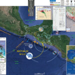
Earlier today there was a moderate sized earthquake (M 6.0) along coast of Ecuador. This earthquake happened in the region of the 2016.04.16 M 7.8 subduction zone earthquake. Based upon the depth and our knowledge of this region, this earthquake may also be on the megathrust. However, the depth is poorly resolved (initially depth ~ 7 km, but now set at 10 km, the default depth). Here is the USGS website for this earthquake.
More information about this earthquake can be found here at earthquake report dot com.
Below is my interpretive poster for this earthquake.
I plot the seismicity from the past month, with color representing depth and diameter representing magnitude (see legend).
- I placed a moment tensor / focal mechanism legend on the poster. There is more material from the USGS web sites about moment tensors and focal mechanisms (the beach ball symbols). Both moment tensors and focal mechanisms are solutions to seismologic data that reveal two possible interpretations for fault orientation and sense of motion. One must use other information, like the regional tectonics, to interpret which of the two possibilities is more likely.
- I also include the shaking intensity contours on the map. These use the Modified Mercalli Intensity Scale (MMI; see the legend on the map). This is based upon a computer model estimate of ground motions, different from the “Did You Feel It?” estimate of ground motions that is actually based on real observations. The MMI is a qualitative measure of shaking intensity. More on the MMI scale can be found here and here. This is based upon a computer model estimate of ground motions, different from the “Did You Feel It?” estimate of ground motions that is actually based on real observations.
- I include the slab contours plotted (Hayes et al., 2012), which are contours that represent the depth to the subduction zone fault. These are mostly based upon seismicity. The depths of the earthquakes have considerable error and do not all occur along the subduction zone faults, so these slab contours are simply the best estimate for the location of the fault.
I include some inset figures in the poster.
- In the lower left corner I include a clipping of the map and cross section from the USGS Open File Report for the historic seismicity of this region (Rhea et al., 2010). I include the seismicity cross section in the upper left corner. This cross section shows earthquakes related to the downgoing Nazca plate.
- Between the map and cross section, I include the MMI intensity maps for both the M 7.8 earthquake and this M 6.0 earthquake.
- In the upper right corner, I include a map that shows the regional tectonics as published by Gutscher et al. (1999). These authors pose that the Carnegie Ridge exerts a control for the segmentation of the subduction zone.
- In the lower right corner, I include a figure from Chlieh et al. (2014) that shows their coupling model. This model informs us about how strongly the subduction zone fault is seismogenically “locked” and how this varies spatially. They also plot historical earthquake locations and their “moment rate deficit” calculation (i.e. how much the plate motion rate has been accumulated as tectonic strain, which would presumably lead to earthquake slip). I include blue stars in the general location of these two earthquakes. The M 7.8 lies within the seismic gap hypothesized by Chlieh et al. (2014).

- Here is the same poster but only with the seismicity from the past month and the MMI contours from the 2016 M 7.8 earthquake. (wait for now to get this done… need to restart software)
- Here are my two interpretive posters for the 2016 M 7.8 earthquake. Here is my initial report. Here is my update.
- First is the initial interpretive poster.

- Here is the updated interpretive poster.
- Below is the tectonic setting map from Gutscher et al. (1999). I include their figure caption as a blockquote.

Tectonic setting of the study area showing major faults, relative plate motions according to GPS data [7] and the NUVEL-1 global kinematic model [8], magnetic anomalies [13] and active volcanoes [50]. Here and in Fig. 4, the locations of the 1906 (Mw D 8:8, very large open circle) and from south to north, the 1953, 1901, 1942, 1958 and 1979 (M 7:8, large open circles) earthquakes are shown. GG D Gulf of Guayaquil; DGM D Dolores–Guayaquil Megashear.
- The 2016 M 7.8 earthquake is near two historic earthquakes with similar magnitudes. Below I plot a map showing the seismicity from 1900-2016 for earthquakes with magnitudes greater than or equal to M 6.0. Here is the USGS query that I used to make this map.
- 1906.01.31 M 8.3 occurred ~100 km to the northeast.
- 1942.05.14 M 7.8 occurred <50 km to the southwest.
- Here are a couple maps from Chlieh et al. (2014). I include their figure captions below. Chlieh et al. (2014) use GPS data to infer the spatial variation and degree to which the subduction zone megathrust is seismogenically coupled. They consider plate motion rates and estimate the moment (earthquake energy) deficit along this fault (how much strain that plate convergence has imparted upon the fault over time). Then they compare this moment deficit to regions of the fault that have slipped historically.
- Tectonics and GPS motion rates.

Seismotectonic setting of the oceanic Nazca plate, South America Craton (SoAm) and two slivers: the North Andean Sliver (NAS) and the Inca Sliver (IS). The relative Nazca/SoAm plate convergence rate in Ecuador is about 55mm/yr (Kendrick et al., 2003). Black arrows indicate the diverging forearc slivers motions relative to stable SoAm are computed from the pole solutions of Nocquet et al.(2014). The NAS indicates a northeastward long-term rigid motion of about 8.5 ±1mm/yr. The ellipse indicates the approximate rupture of the great 1906 Mw=8.8 Colombia–Ecuador megathrust earthquake. The Carnegie Ridge intersects the trench in central Ecuador and coincides with the southern limit of the great 1906 event. Plate limits (thick red lines) are from Bird(2003). DGFZ =Dolores–Guayaquil Fault Zone; GG =Gulf of Guayaquil; GR =Grijalva Ridge; AR =Alvarado Ridge; SR =Sarmiento Ridge. (For interpretation of the references to color in this figure legend, the reader is referred to the web version of this article.)
- GPS velocities along with historic earthquake patches.

Interseismic GPS velocity field in the North Andean Sliver reference frame. The relative Nazca/NAS convergence rate is 46 mm/yr. The highest GPS velocity of 26 mm/yr is found on La Plata Island that is the closest point to the trench axis. The GPS network adequately covers the rupture areas of the 1998 Mw=7.1, 1942 Mw=7.8and 1958 Mw=7.7 earthquakes but only 1/4th of the 1979 Mw=8.2 and 2/3rd of the great 1906 Mw=8.8 rupture area. The black star is the epicenter of the great 1906 event and white stars are the epicenters of the Mw>7.01942–1998 seismic sequence. Grey shaded ellipses are the high slip region of the 1942, 1958, 1979 and 1998 seismic sources (Beck and Ruff, 1984;Segovia, 2001; Swenson and Beck, 1996). Red dashed contours are the relocated aftershocks areas of the 1942, 1958 and 1979 events (Mendoza and Dewey, 1984). (For interpretation of the references to color in this figure legend, the reader is referred to the web version of this article.)
- Moment deficit along strike and historic earthquake locations (Chlieh et al., 2014). The 2016 M 7.8 earthquake may have occurred in the region marked “gap” in these figures.

(A) Along-strike variations of the annual moment deficit for all the interseismic models shown in Fig.5. (B)Maximum ISC model and (C)Minimum ISC model. (A)The blue, green and red lines correspond to the along-strike variation of the annual moment deficit rate respectively for models with smoothing coefficient λ1 =1.0, 0.25 and 0.1. (B) Smoother solution of Fig.5 ith a maximum moment deficit rate of 4.5 ×10¹⁸N m/yr. (C)Rougher solution of Fig.5 with a minimum moment deficit rate of 2.5 ×10¹⁸N m/yr. Yellow stars are the epicenters of subduction earthquakes with magnitude Mw>6.0 from the last 400 yr catalogue (Beauval et al., 2013). (For interpretation of the references to color in this figure legend, the reader is referred to the web version of this article.)
References
- Chlieh, M. Mothes, P.A>, Nocquet, J-M., Jarrin, P., Charvis, P., Cisneros, D., Font, Y., Color, J-Y., Villegas-Lanza, J-C., Rolandone, F., Vallée, M., Regnier, M., Sogovia, M., Martin, X., and Yepes, H., 2014. Distribution of discrete seismic asperities and aseismic slip along the Ecuadorian megathrust in Earth and Planetary Science Letters, v. 400, p. 292–301
- Gutscher, M-A., Malavieille, J., Lallemand, S., and Collor, J-Y., 1999. Tectonic segmentation of the North Andean margin: impact of the Carnegie Ridge collision in Earth and Planetary Science Letters, v.168, p. 255–270
- Hayes, G. P., D. J. Wald, and R. L. Johnson, 2012. Slab1.0: A three-dimensional model of global subduction zone geometries, J. Geophys. Res., 117, B01302, doi:10.1029/2011JB008524.
- Rhea, Susan, Hayes, Gavin, Villaseñor, Antonio, Furlong, K.P., Tarr, A.C., and Benz, H.M., 2010. Seismicity of the earth 1900–2007, Nazca Plate and South America: U.S. Geological Survey Open-File Report 2010–1083-E, 1 sheet, scale 1:12,000,000.
This morning we had an earthquake offshore of Guatemala with a magnitude M = 6.8. Here is the USGS website for this earthquake. This earthquake occurred to the east of a sequence from about a week ago. Here is my earthquake report for that sequence.
Offshore of Guatemala is a subduction zone thrust fault, where the Cocos plate dives east beneath the North America (in the north) and Caribbean plates (in the south). Subduction zone faults are capable of generating the largest magnitude earthquakes possible because the fault width is wider than other faults. The seismogenic zone, the region of the crust that can store elastic strain and experience brittle rupture during earthquakes, extends into the earth several tens of kms. Strike-slip faults generally dip vertically, giving them the narrowest fault width. While subduction zones dip at an angle, so their fault width is wider. Earthquake magnitude is a measure of energy released during the earthquake and the moment magnitude (the magnitude most people use) is based on three factors: (1) fault area, (2) fault slip, and (3) shear modulus (how flexible, or rigid, the crust/lithosphere is). Fault area is length times width. Length is the distance on the ground surface that the fault ruptures and width is the distance into the earth that the fault ruptures. Because subduction zone faults dip into the earth at an angle, the distance that they extend before reaching a given depth is larger, owing to a larger possible magnitude.
Today’s M 6.8 earthquake has a USGS hypocentral depth of ~47 km, which is very close to the depth of the subduction zone fault. Also, the fault plane solution (moment tensor, read below) is compressional. Thus, I interpret this earthquake to be a subduction zone earthquake at or near the megathrust. This earthquake is different from the sequence from a week ago. Those earthquakes had two populations: (1) earthquakes in the accretionary prism of the subduction zone and (2) earthquakes in the downgoing Cocos plate. Those earthquakes were not subduction zone earthquakes (though the shallower earthquakes may not have had well located hypocenters, so their depths are suspect… and could have been on the subduction zone). I suspect that this M 6.8 earthquake is related to the earthquakes from last week. I include the moment tensors for 2 of the significant earthquakes from last week. See my report for more on that sequence.
Below is my interpretive poster for this earthquake.
I plot the seismicity from the past month, with color representing depth and diameter representing magnitude (see legend).
- I placed a moment tensor / focal mechanism legend on the poster. There is more material from the USGS web sites about moment tensors and focal mechanisms (the beach ball symbols). Both moment tensors and focal mechanisms are solutions to seismologic data that reveal two possible interpretations for fault orientation and sense of motion. One must use other information, like the regional tectonics, to interpret which of the two possibilities is more likely.
- I also include the shaking intensity contours on the map. These use the Modified Mercalli Intensity Scale (MMI; see the legend on the map). This is based upon a computer model estimate of ground motions, different from the “Did You Feel It?” estimate of ground motions that is actually based on real observations. The MMI is a qualitative measure of shaking intensity. More on the MMI scale can be found here and here. This is based upon a computer model estimate of ground motions, different from the “Did You Feel It?” estimate of ground motions that is actually based on real observations.
- I include the slab contours plotted (Hayes et al., 2012), which are contours that represent the depth to the subduction zone fault. These are mostly based upon seismicity. The depths of the earthquakes have considerable error and do not all occur along the subduction zone faults, so these slab contours are simply the best estimate for the location of the fault. The hypocentral depth of the M 6.8 plots this close to the location of the fault as mapped by Hayes et al. (2012).
I include some inset figures in the poster.
- In the upper right corner, I include a subset of figures from Benz et al. (2011). There is a map that shows USGS epicenters with dots colored by depth and magnitude represented by circle diameter. There is also plotted a cross section that is adjacent (southeast) to this earthquake sequence. Cross section B-B’ shows the earthquake hypocenters along a profile displayed on the map. Note how the subduction zone dip steepens to the northeast. On the map and the cross section, I place a blue stars in the location for the M 6.9 and the 6/14 M 5.5 earthquakes.
- In the lower right corner is a tectonic map showing the regional tectonics highlighting various study sites from sedimentary, magmatic, metamorphic and ore deposit studies of the subduction zones here (Garcia-Casco et al., 2011).
- In the lower left corner is a map that shows the plate tectonic setting for this region of Middle America (Symithe et al., 2015). Earthquake epicenters are plotted as circles with color representing depth. Earthquake focal mechanisms are plotted with thrust earthquakes plotted in blue and other mechanisms plotted in red. Today’s earthquake happened just off this map on the left.

- Here is an explanation from IPGP that helps us visualize the two potential fault planes (the principal and the auxiliary). I interpret this earthquake to have occurred on fault plane 1, the subduction zone.
- Here is a map that shows today’s earthquake (with MMI contours) in the context of the seismicity from the past 100 years. I plot earthquakes from 1917-2017 for magnitudes M > 6.5.
- Here is my poster for the earthquake sequence from last week.
- Here is the tectonic map from Symithe et al. (2015). I include their figure caption below in blockquote.

Seismotectonic setting of the Caribbean region. Black lines show the major active plate boundary faults. Colored circles are precisely relocated seismicity [1960–2008, Engdahl et al., 1998] color coded as a function of depth. Earthquake focal mechanism are from the Global CMT Catalog (1976–2014) [Ekstrom et al., 2012], thrust focal mechanisms are shown in blue, others in red. H = Haiti, DR = Dominican Republic, MCS = mid-Cayman spreading center, WP = Windward Passage, EPGF = Enriquillo Plaintain Garden fault.
- Here is the tectonic map from Garcia-Casco et al. (2011). I include their figure caption below in blockquote.

Plate tectonic configuration of the Caribbean region showing the location of the study cases presented in this issue (numbers refer to papers, arranged as in the issue), and other important geological features of the region (compiled from several sources).
- Here is the Benz et al. (2011) Seismicity of the Earth poster for this region.
References
- Benz, H.M., Tarr, A.C., Hayes, G.P., Villaseñor, Antonio, Furlong, K.P., Dart, R.L., and Rhea, Susan, 2011. Seismicity of the Earth 1900–2010 Caribbean plate and vicinity: U.S. Geological Survey Open-File Report 2010–1083-A, scale 1:8,000,000.
- Franco, A., C. Lasserre H. Lyon-Caen V. Kostoglodov E. Molina M. Guzman-Speziale D. Monterosso V. Robles C. Figueroa W. Amaya E. Barrier L. Chiquin S. Moran O. Flores J. Romero J. A. Santiago M. Manea V. C. Manea, 2012. Fault kinematics in northern Central America and coupling along the subduction interface of the Cocos Plate, from GPS data in Chiapas (Mexico), Guatemala and El Salvador in Geophysical Journal International., v. 189, no. 3, p. 1223-1236. DOI: https://doi.org/10.1111/j.1365-246X.2012.05390.x
- Garcia-Casco, A., Projenza, J.A., Iturralde-Vinent, M.A., 2011. Subduction Zones of the Caribbean: the sedimentary, magmatic, metamorphic and ore-deposit records UNESCO/iugs igcp Project 546 Subduction Zones of the Caribbean in Geologica Acta, v. 9, no., 3-4, p. 217-224
- Hayes, G. P., D. J. Wald, and R. L. Johnson, 2012. Slab1.0: A three-dimensional model of global subduction zone geometries, J. Geophys. Res., 117, B01302, doi:10.1029/2011JB008524.
- Symithe, S., E. Calais, J. B. de Chabalier, R. Robertson, and M. Higgins, 2015. Current block motions and strain accumulation on active faults in the Caribbean in J. Geophys. Res. Solid Earth, v. 120, p. 3748–3774, doi:10.1002/2014JB011779.
There was a really cool earthquake sequence a few days ago on and offshore of Guatemala. Offshore of Guatemala in the Pacific Ocean, the Cocos plate subducts beneath the North America and Caribbean plates (NAP & CP). The transform plate boundary between the NAP and CP forms the Motagua-Polochic fault zone onshore, which bisects Guatemala.
From late May 2017 through mid June there were several earthquakes with the largest magnitude M = 5.5. These earthquake hypocenters have depths that are deeper and shallower than the estimated depth for the subduction zone fault (Hayes et al., 2012), but many of the earthquakes simply have a default depth of 10 km. So it is difficult to say if these are all near the megathrust or are on upper plate faults (e.g. in the accretionary prism). These earthquakes have compressional fault plane solutions. Either way, they appear to have loaded some faults down-dip along the subducting slab. This may or may not be the case, but there was a deep extensional magnitude M 6.9 earthquake (with an aftershock of M = 5.1 nearby). These along dip earthquakes are probably related.
Below is my interpretive poster for this earthquake.
I plot the seismicity from the past month, with color representing depth and diameter representing magnitude (see legend).
- I placed a moment tensor / focal mechanism legend on the poster. There is more material from the USGS web sites about moment tensors and focal mechanisms (the beach ball symbols). Both moment tensors and focal mechanisms are solutions to seismologic data that reveal two possible interpretations for fault orientation and sense of motion. One must use other information, like the regional tectonics, to interpret which of the two possibilities is more likely.
- I also include the shaking intensity contours on the map. These use the Modified Mercalli Intensity Scale (MMI; see the legend on the map). This is based upon a computer model estimate of ground motions, different from the “Did You Feel It?” estimate of ground motions that is actually based on real observations. The MMI is a qualitative measure of shaking intensity. More on the MMI scale can be found here and here. This is based upon a computer model estimate of ground motions, different from the “Did You Feel It?” estimate of ground motions that is actually based on real observations.
- I include the slab contours plotted (Hayes et al., 2012), which are contours that represent the depth to the subduction zone fault. These are mostly based upon seismicity. The depths of the earthquakes have considerable error and do not all occur along the subduction zone faults, so these slab contours are simply the best estimate for the location of the fault. The hypocentral depth of the M 5.5 plots this close to the location of the fault as mapped by Hayes et al. (2012).
I include some inset figures in the poster.
- In the upper right corner, I include a subset of figures from Benz et al. (2011). There is a map that shows USGS epicenters with dots colored by depth and magnitude represented by circle diameter. There is also plotted a cross section that is adjacent (southeast) to this earthquake sequence. Cross section B-B’ shows the earthquake hypocenters along a profile displayed on the map. Note how the subduction zone dip steepens to the northeast. On the map and the cross section, I place a blue stars in the location for the M 6.9 and the 6/14 M 5.5 earthquakes.
- To the left of these figures is a comparison map and plot, showing the responses from real people who reported their observations during these two earthquakes. Below each map are plotted the reports from the Did You Feel It? USGS website for each earthquake. These reports are plotted as green dots with intensity on the vertical axes and distance on the horizontal axes. There are comparisons with Ground Motion Prediction Equation (attenuation relations) results (the orange model uses empirical data from central and eastern US earthquakes; the green model uses empirical data from earthquakes in California). The M 5.5 earthquake seems to fit the Central-Eastern US regression much better than the California regression. However, there are very few observations. The M 6.9 earthquake seems to fit the California regression better.
- In the lower left corner is a map that shows the plate tectonic setting for this region of Middle America (Eric Calias). Earthquake epicenters are plotted with color representing depth and circle diameter representing magnitude. Dr. Calais shaded the Caribbean plate a little darker than the surrounding plates. Relative plate motions are plotted as white arrows. I place a blue star in the general location of the M 6.9 earthquake.
- Above the tectonic figure, is a figure that shows how Franco et al. (2012) hypothesize that the amount that the subducting fault is locked (“coupling” or the proportion of the plate convergence rate that is stored along the fault that would eventually slip during earthquakes). Note that this earthquake sequence mostly occurred in the segment of the subduction zone that has high coupling. I place a blue star in the general location of the M 6.9 earthquake.
- In the lower right corner I plot most all the available moment tensors for the earthquakes in this sequence. I label the Polochic and Motagua faults that delineate the Motagua-Polochic fault zone, left lateral strike-slip faults that form the boundary between the Caribbean and North America plates.

Here are the USGS webpages for the earthquakes with moment tensors plotted above
- Here is the USGS Did You Feel It comparison.
References
- Benz, H.M., Tarr, A.C., Hayes, G.P., Villaseñor, Antonio, Furlong, K.P., Dart, R.L., and Rhea, Susan, 2011. Seismicity of the Earth 1900–2010 Caribbean plate and vicinity: U.S. Geological Survey Open-File Report 2010–1083-A, scale 1:8,000,000.
- Eric Calias, Purdue University
- Franco, A., C. Lasserre H. Lyon-Caen V. Kostoglodov E. Molina M. Guzman-Speziale D. Monterosso V. Robles C. Figueroa W. Amaya E. Barrier L. Chiquin S. Moran O. Flores J. Romero J. A. Santiago M. Manea V. C. Manea, 2012. Fault kinematics in northern Central America and coupling along the subduction interface of the Cocos Plate, from GPS data in Chiapas (Mexico), Guatemala and El Salvador in Geophysical Journal International., v. 189, no. 3, p. 1223-1236. DOI: https://doi.org/10.1111/j.1365-246X.2012.05390.x
- Hayes, G. P., D. J. Wald, and R. L. Johnson, 2012. Slab1.0: A three-dimensional model of global subduction zone geometries, J. Geophys. Res., 117, B01302, doi:10.1029/2011JB008524.
This earthquake happened a couple weeks ago, but was interesting and I have been looking forward to following up on this with a report. Here is the USGS website for this M 6.8 earthquake.
The M 6.8 earthquake happened in a region where the Pacific-North America plate boundary transitions from a subduction zone to a shear zone. To the east of this region, the Pacific plate subducts beneath the North America plate to form the Alaska-Aleutian subduction zone. As a result of this subduction, a deep oceanic trench is formed. To the west of this earthquake, the plate boundary is in the form of a shear zone composed of several strike-slip faults. The main fault that is positioned in the trench is the Bering-Kresla shear zone (BKSZ), a right-lateral strike-slip fault. In the oceanic basin to the north of the BKSZ there are a series of parallel fracture zones, also right-lateral strike-slip faults.
My initial thought is that the entire Aleutian trench was a subduction zone prior to about 47 million years ago (Wilson, 1963; Torsvik et al., 2017). Prior to 47 Ma, the relative plate motion in the region of the BKSZ would have been more orthogonal (possibly leading to subduction there). After 47 Ma, the relative plate motion in the region of the BKSZ has been parallel to the plate boundary, owing to the strike-slip motion here. However, Konstantinovskaia (2001) used paleomagnetic data for a plate motion reconstruction through the Cenozoic and they have concluded that there is a much more complicated tectonic history here (with strike-slip faults in the region prior to 47 Ma and other faults extending much farther east into the plate boundary). When considering this, I was reminded that the relative plate motion in the central Aleutian subduction zone is oblique. This results in strain partitioning where the oblique motion is partitioned into fault-normal fault movement (subduction) and fault-parallel fault movement (strike-slip, along forearc sliver faults). The magmatic arc in the central Aleutian subduction zone has a forearc sliver fault, but also appears to have blocks that rotate in response to this shear (Krutikov, 2008).
There have been several other M ~6 earthquakes to the west that are good examples of this strike-slip faulting in this area. On 2003.12.05 there was a M 6.7 earthquake along the Bering fracture zone (the first major strike-slip fault northeast of the BKSZ). On 2016.09.05 there was a M 6.3 earthquake also on the Bering fracture zone. Here is my earthquake report for the 2016 M 6.3 earthquake. The next major strike-slip fault, moving away from the BKSZ, is the right-lateral Alpha fracture zone. The M 6.8 earthquake may be related to this northwest striking fracture zone. However, aftershocks instead suggest that this M 6.8 earthquake is on a fault oriented in the northeast direction. There is no northeast striking strike-slip fault mapped in this area and the Shirshov Ridge is mapped as a thrust fault (albeit inactive). There is a left-lateral strike-slip fault that splays off the northern boundary of Bowers Ridge. If this fault strikes a little more counter-slockwise than is currently mapped at, the orientation would match the fault plane solution for this M 6.8 earthquake (and also satisfies the left-lateral motion for this orientation). The bathymetry used in Google Earth does not reveal the orientation of this fault, but the aftershocks sure align nicely with this hypothesis.
Below is my interpretive poster for this earthquake.
I plot the seismicity from the past month, with color representing depth and diameter representing magnitude (see legend). I also include USGS earthquake epicenters from 1997-2017 for magnitudes M ≥ 6.5.
- I placed a moment tensor / focal mechanism legend on the poster. There is more material from the USGS web sites about moment tensors and focal mechanisms (the beach ball symbols). Both moment tensors and focal mechanisms are solutions to seismologic data that reveal two possible interpretations for fault orientation and sense of motion. One must use other information, like the regional tectonics, to interpret which of the two possibilities is more likely. I plot moment tensors for the M 6.8 earthquake, as well as for the 2003 and 2016 earthquakes mentioned above. I also include moment tensors for earthquakes in 1999 and 2001 because these are also interesting earthquakes that I had not noticed before. It appears that perhaps the 1999 strike-slip earthquake led to an increased stress on the subduction zone, which slipped in 2001. I will need to consider this earthquake pair more later. Here are the USGS websites for the 1999 and 2001 earthquakes.
- I also include the shaking intensity contours on the map. These use the Modified Mercalli Intensity Scale (MMI; see the legend on the map). This is based upon a computer model estimate of ground motions, different from the “Did You Feel It?” estimate of ground motions that is actually based on real observations. The MMI is a qualitative measure of shaking intensity. More on the MMI scale can be found here and here. This is based upon a computer model estimate of ground motions, different from the “Did You Feel It?” estimate of ground motions that is actually based on real observations.
- I include the slab contours plotted (Hayes et al., 2012), which are contours that represent the depth to the subduction zone fault. These are mostly based upon seismicity. The depths of the earthquakes have considerable error and do not all occur along the subduction zone faults, so these slab contours are simply the best estimate for the location of the fault. The hypocentral depth of the M 5.5 plots this close to the location of the fault as mapped by Hayes et al. (2012).
I include some inset figures in the poster.
- In the upper right corner is a figure that shows the historic earthquake ruptures along the Aleutian Megathrust (Peter Haeussler, USGS). I place a yellow star in the general location of this earthquake sequence (same for other figures here).
- In the upper left corner is a figure from Gaedicke et al. (2000) which shows some of the major tectonic faults in this region.
- In the lower right corner is a figure from Konstantnovskaia et al. (2001) that shows a very detailed view of all the faults in this complicated region.

- On 2017.05.08 there was an earthquake further to the east, with a magnitude M 6.2. Here is my interpretive poster for this earthquake, which includes fault plane solutions for several historic earthquakes in the region. These fault plane solutions reveal the complicated intersection of these two different types of faulting along this plate boundary. Here is my earthquake report for this earthquake sequence.
- Here is a map that shows some of the large earthquakes in this region from 1996 through 2015. Refer to the moment tensor legend to help interpret the moment tensors for each earthquake. All, but one, are compressional solutions. Note how all the compressional earthquakes have roughly the same strike, oriented relative to the plate convergence vectors (blue arrows). Note the fault plane solution and location for the 2014.06.23 M 7.2 earthquake. Do we see a trend here? This earthquake suggests the strike-slip faulting extends at least to the Bowers Ridge.
- Here is a map that shows historic earthquake slip regions as pink polygons (Peter Haeussler, USGS). Dr. Haeussler also plotted the magnetic anomalies (grey regions), the arc volcanoes (black diamonds), and the plate motion vectors (mm/yr, NAP vs PP).
- Here are several figures from Gaedicke et al. (2000) showing their tectonic reconstructions. I include their figure captions below in blockquote. The first map shows the general tectonic setting as in the poster above.

Map of the Aleutian–Bering region and location of the study area (rectangle). Lines with barbs indicate subduction zones: (1) Kamchatka Trench and (2) Aleutian Trench; lines with sense of displacement mark fracture zones (FZs): (3) Steller, (4) Pikezh and (5) Bering FZs. Single arrows show relative direction of convergence of the Pacific (P) and North American (NA) plates. Bathymetric contours are in meters.
- This figure shows the complicated intersection of the BKSZ and the Kuril-Kamchatka Trench (a subduction zone).

The main tectonic features of the Kamchatka–Aleutian junction area modified from Seliverstov (1983), Seliverstov et al. (1988) and Baranov et al. (1991). The eastern side of the Central Kamchatka depression is bounded by normal faults. Contour interval is 1000 m. Lines A and B indicate the locations of profiles shown in Fig. 3; the rectangle marks the location of the area shown in Fig. 4.
- This figure shows a medium scale view of the faults here, along with the major historic earthquakes. In this figure the BKSZ is labeled the Aleutian fracture zone (AFZ).

Rupture zones of the major earthquakes in the Kamchatka–Aleutian junction area [according to Vikulin (1997)]. Earthquakes with a magnitude of Mw>7 are shown.
- Here is a figure from Krutikov (2008) showing the block rotation and forearc sliver faults associated with the oblique subduction in the central Aleutian subduction zone. Note that there are blocks that are rotating to accommodate the oblique convergence. There are also margin parallel strike slip faults that bound these blocks. These faults are in the upper plate, but may impart localized strain to the lower plate, resulting in strike slip motion on the lower plate (my arm waving part of this). Note how the upper plate strike-slip faults have the same sense of motion as these deeper earthquakes.
- Here is a figure that shows the plate age for seamounts in the Hawaii-Emperor Seamount Chain (Torsvik et al., 2017).

Hawaiian-Emperor Chain. White dots are the locations of radiometrically dated seamounts, atolls and islands, based on compilations of Doubrovine et al. and O’Connor et al. Features encircled with larger white circles are discussed in the text and Fig. 2. Marine gravity anomaly map is from Sandwell and Smith.
- Here are several figures from Konstantnovskaia et al. (2001) showing their tectonic reconstructions. I include their figure captions below in blockquote. The first figure is the one included in the poster above.

Geodynamic setting of Kamchatka in framework of the Northwest Pacific. Modified after Nokleberg et al. (1994) and Kharakhinov (1996)). Simplified cross-section line I-I’ is shown in Fig. 2. The inset shows location of Sredinny and Eastern Ranges. [More figure caption text in the publication].
- Here are 4 panels that show the details of their reconstructions. Panels shown are for 65 Ma, 55 Ma, 37 Ma, and Present.


The Cenozoic evolution in the Northwest Pacific. Plate kinematics is shown in hotspot reference frame after (Engebretson et al., 1985). Keys distinguish zones of active volcanism (thick black lines), inactive volcanic belts (thick gray lines), deformed arc terranes (hatched pattern), subduction zones: active (black triangles), inactive *(empty triangles). In letters: sa = Sikhote-aline, bs = Bering shelf belts; SH = Shirshov Ridge; V = Vitus arch; KA = Kuril; RA = Ryukyu’ LA = Luzon; IBMA = Izu-Bonin-Mariana arcs; WPB = Western Philippine, BB = Bowers basins.
Alaska | Kamchatka | Kurile
Earthquake Reports
2017.06.02 M 6.8 Aleutians
2017.05.08 M 6.2 Aleutians
2017.05.01 M 6.3 British Columbia
2017.03.29 M 6.6 Kamchatka
2017.03.02 M 5.5 Alaska
2016.09.05 M 6.3 Bering Kresla (west of Aleutians)
2016.04.02 M 6.2 Alaska Peninsula
2016.03.27 M 5.7 Aleutians
2016.03.12 M 6.3 Aleutians
2016.01.24 M 7.1 Alaska
2015.11.09 M 6.2 Aleutians
2015.11.02 M 5.9 Aleutians
2015.11.02 M 5.9 Aleutians (update)
2015.07.27 M 6.9 Aleutians
2015.05.29 M 6.7 Alaska Peninsula
2015.05.29 M 6.7 Alaska Peninsula (animations)
1964.03.27 M 9.2 Good Friday
References
- Gaedicke, C., Baranov, B., Seliverstov, N., Alexeiev, D., Tsukanov, N., Freitag, R., 2000. Structure of an active arc-continent collision area: the Aleutian-Kamchatka junction. Tectonophysics 325, 63–85
- Hayes, G. P., D. J. Wald, and R. L. Johnson, 2012. Slab1.0: A three-dimensional model of global subduction zone geometries, J. Geophys. Res., 117, B01302, doi:10.1029/2011JB008524.
- Konstantnovskaia, 2001. Arc-continent collision and subduction reversal in the Cenozoic evolution of the Northwest Pacific: an example from Kamchatka (NE Russia) in Tectonophysics, v. 333, p. 75-94.
- Krutikov, L., et al., 2008. Active Tectonics and Seismic Potential of Alaska, Geophysical Monograph Series 179, doi:10.1029/179GM07
- Lange, D., Cembrano, J., Rietbrock, A., Haberland, C., Dahm, T., and Bataille, K., 2008. First seismic record for intra-arc strike-slip tectonics along the Liquiñe-Ofqui fault zone at the obliquely convergent plate margin of the southern Andes in Tectonophysics, v. 455, p. 14-24
- Torsvik, T. H. et al., 2017. Pacific plate motion change caused the Hawaiian-Emperor Bend in Nat. Commun., v. 8, doi: 10.1038/ncomms15660
- Wilson, J. Tuzo, 1963. “A possible origin of the Hawaiian Islands” in Canadian Journal of Physics. v. 41, p. 863–870 doi:10.1139/p63-094.
We had a couple of earthquakes in western Turkey today (in the Aegean Sea offshore of the Island of Lesbos, part of Greece). The M 6.3 earthquake shows evidence for extension (normal fault), based on the moment tensor (read below).
The tectonics here are dominated by the compressional tectonics related to (1) the Alpide Belt, a convergent plate boundary formed in the Cenozoic that extends from Australia to Morocco and (2) the North Anatolia fault, a strike-slip fault system that strikes along northern Turkey and extends into Greece and the Aegean Sea.
There is a series of normal faults in this region of the north Aegean Sea and today’s earthquakes are likely associated with that extensional regime. The M 6.3 epicenter plots near the Magiras fault, though the strike of the fault is different from the orientation of the moment tensor. Perhaps the fault is not optimally aligned to the modern tectonic strain. There was an earthquake on 1949.07.23 that had a similarly oriented fault plane solution (showing northeast-southwest extension), which probably occurred on the Northern Chios fault. See below (Papazachos et al., 1998).
Below is my interpretive poster for this earthquake.
I plot the seismicity from the past month, with color representing depth and diameter representing magnitude (see legend). I also include USGS seismicity from 1917-2017 for earthquakes with M ≥ 6.0.
- I placed a moment tensor / focal mechanism legend on the poster. There is more material from the USGS web sites about moment tensors and focal mechanisms (the beach ball symbols). Both moment tensors and focal mechanisms are solutions to seismologic data that reveal two possible interpretations for fault orientation and sense of motion. One must use other information, like the regional tectonics, to interpret which of the two possibilities is more likely.
- I also include the shaking intensity contours on the map. These use the Modified Mercalli Intensity Scale (MMI; see the legend on the map). This is based upon a computer model estimate of ground motions, different from the “Did You Feel It?” estimate of ground motions that is actually based on real observations. The MMI is a qualitative measure of shaking intensity. More on the MMI scale can be found here and here. This is based upon a computer model estimate of ground motions, different from the “Did You Feel It?” estimate of ground motions that is actually based on real observations.
- I include faults included in two fault databases. Faults in Italy are from the Instituto Nazionale di Geofisica e Vulcanologia Database of Individual Seismogenic Sources (DISS; Basili et al., 2008; DISS Working Group, 2015). This DISS is available online here. The faults in Greece are from the Greek Satabase of Seismogenic Sources (GreDaSS; Caputo et al., 2012). The GreDaSS is available online here.
I include some inset figures in the poster.
- In the upper right corner is a regional tectonic map from Dilek and Sandvol (2009). This shows all the major tectonic plate boundary faults, as well as some of the major intraplate faults for this region. Reverse/Thrust faults are labeled with triangles on the upthrown (hanging wall) side of the fault. strike slip faults show relative motion arrows on either sides of the fault. The different plates and microplates are colored. I place a cyan star in the general location of today’s earthquake (also placed in the other inset figures).
- In the upper left corner is a map that shows focal mechanisms for historic earthquakes in this region. Note the focal mechanism for the 1949 earthquake and compare this with the M 6.3 earthquake moment tensor from today.
- In the lower right corner I include a larger scale view of the seismicity and faults displayed in the main map. I here also include the fault planes from the active fault databases (orange rectilinear polygons). These polygons show how different faults dip in different directions. The strike slip faults have more narrow polygons becuase they dip more vertically than the normal and thrust/reverse faults. I label the two faults mentioned above (possibly related to the 2017 M 6.3 and 1949 M 6.5 earthquakes), the Magiras and Northern Chios faults (Caputo et al., 2012).
- In the lower left corner is a figure from Ersoy et al. (2014). This shows their interpretation of the geodynamics of the Aegean Sea. They hypothesize that this region is rotating in a clockwise fashion, leading to extension in western Turkey and the northern Aegean Sea. The 1949 and 2017 earthquake fault plane solutions (focal mechanisma and moment tensors) are oriented correctly with this model.

- Here is the tectonic map from Dilek and Sandvol (2009).

Tectonic map of the Aegean and eastern Mediterranean region showing the main plate boundaries, major suture zones, fault systems and tectonic units. Thick, white arrows depict the direction and magnitude (mm a21) of plate convergence; grey arrows mark the direction of extension (Miocene–Recent). Orange and purple delineate Eurasian and African plate affinities, respectively. Key to lettering: BF, Burdur fault; CACC, Central Anatolian Crystalline Complex; DKF, Datc¸a–Kale fault (part of the SW Anatolian Shear Zone); EAFZ, East Anatolian fault zone; EF, Ecemis fault; EKP, Erzurum–Kars Plateau; IASZ, Izmir–Ankara suture zone; IPS, Intra–Pontide suture zone; ITS, Inner–Tauride suture; KF, Kefalonia fault; KOTJ, Karliova triple junction; MM, Menderes massif; MS, Marmara Sea; MTR, Maras triple junction; NAFZ, North Anatolian fault zone; OF, Ovacik fault; PSF, Pampak–Sevan fault; TF, Tutak fault; TGF, Tuzgo¨lu¨ fault; TIP, Turkish–Iranian plateau (modified from Dilek 2006).
- Here is a great map from Ersoy et al. (2014) that shows the geologic map of the region. Faults are shown also. Today’s earthquakes happened in the northwest corner of the figure 2 inset rectangle.

Tectonostratigraphic units and major tectonic elements of the Aegean Extensional Province (compiled from1/500,000 scaled geological maps of Greece (IGME) and Turkey (MTA), Okay and Tüysüz, 1999; Ring et al., 2001, 2010; Candan et al., 2005; van Hinsbergen et al., 2005; Ersoy and Palmer, 2013). CRCC: Central Rhodope, SRCC: Southern Rhodope, KCC: Kazdağ, CCC: Cycladic, SAC: South Aegean (Crete) core complexes. KKD: Kesebir–Kardamos Dome. MEMC1 and MEMC2 refer to first- and second-stage development of theMenderes Extensional Metamorphic Complex (MEMC). VİAS: Vardar–İzmir–Ankara suture zone, NAF: North Anatolian Fault Zone.
- This is the Ersoy et al. (2014) map showing their interpretation of the modern deformation in the northern Aegean Sea and western Turkey.

Geological map showing the distribution of the Menderes Extensional Metamorphic Complex (MEMC), Oligocene–Miocene volcanic and sedimentary units and volcanic centers in the Aegean Extensional Province (compiled from geological maps of Greece (IGME) and Turkey (MTA), and adapted from Ersoy and Palmer, 2013). Extensional deformation field with rotation (rotational extension) is shown with gray field, and simplified from Brun and Sokoutis (2012), Kissel et al. (2003) and van Hinsbergen and Schmid (2012). İzmir–Balıkesir Transfer zone (İBTZ) give the outer limit for the rotational extension, and also limit of ellipsoidal structure of the MEMC. MEMC developed in two stages: the first one was accommodated during early Miocene by the Simav Detachment Fault (SDF) in the north; and the second one developed during Middle Miocene along the Gediz (Alaşehir) Detachment Fault (GDF) and Küçük Menderes Detachment Fault (KMDF). Extensional detachments were also accommodated by strike-slip movement along the İBTZ (Ersoy et al., 2011) and Uşak–Muğla Transfer Zone (Çemen et al., 2006; Karaoğlu and Helvacı, 2012). Other main core complexes in the Aegean, the Central Rhodope (CRCC), Southern Rhodope (SRCC), Kesebir–Kardamos Dome (KKD) and Cycladic (CCC) Core Complexes are also shown. The area bordered with dashed green line represents the surface trace of the asthenospheric window between the Aegean and Cyprean subducted slabs (Biryol et al., 2011; de Boorder et al., 1998). See text for detail.
- This is a great figure showing another interpretation to explain the extension in this region (slab rollback and mantle flow) from Brun and Sokoutis (2012).

Mantle flow pattern at Aegean scale powered by slab rollback in rotation around vertical axis located at Scutary-Pec (Albania). A: Map view of fl ow lines above (red) and below (blue) slab. B: Three-dimensional sketch showing how slab tear may accommodate slab rotation. Mantle fl ow above and below slab in red and blue, respectively. Yellow arrows show crustal stretching.
- The following three figures are from Dilek and Sandvol, 2006. The locations of the cross sections are shown on the map as orange lines. Cross section G-G’ is located in the region of today’s earthquake.
- Here is the map (Dilek and Sandvol, 2006). I include the figure caption below in blockquote.

Simplified tectonic map of the Mediterranean region showing the plate boundaries, collisional zones, and directions of extension and tectonic transport. Red lines A through G show the approximate profile lines for the geological traverses depicted in Figure 2. MHSZ—mid-Hungarian shear zone; MP—Moesian platform; RM—Rhodope massif; IAESZ— Izmir-Ankara-Erzincan suture zone; IPS—Intra-Pontide suture zone; ITS—inner Tauride suture zone; NAFZ—north Anatolian fault zone; KB—Kirsehir block; EKP—Erzurum-Kars plateau; TIP—Turkish-Iranian plateau.
- Here are cross sections A-D (Dilek and Sandvol, 2006). I include the figure caption below in blockquote.


Simplified tectonic cross-sections across various segments of the broader Alpine orogenic belt.
- (A) Eastern Alps. The collision of Adria with Europe produced a bidivergent crustal architecture with both NNW- and SSE-directed nappe structures that involved Tertiary molasse deposits, with deep-seated thrust faults that exhumed lower crustal rocks. The Austro-Alpine units north of the Peri-Adriatic lineament represent the allochthonous outliers of the Adriatic upper crust tectonically resting on the underplating European crust. The Penninic ophiolites mark the remnants of the Mesozoic ocean basin (Meliata). The Oligocene granitoids between the Tauern window and the Peri-Adriatic lineament represent the postcollisional intrusions in the eastern Alps. Modified from Castellarin et al. (2006), with additional data from Coward and Dietrich (1989); Lüschen et al. (2006); Ortner et al. (2006).
- (B) Northern Apennines. Following the collision of Adria with the Apenninic platform and Europe in the late Miocene, the westward subduction of the Adriatic lithosphere and the slab roll-back (eastward) produced a broad extensional regime in the west (Apenninic back-arc extension) affecting the Alpine orogenic crust, and also a frontal thrust belt to the east. Lithospheric-scale extension in this broad back-arc environment above the west-dipping Adria lithosphere resulted in the development of a large boudinage structure in the European (Alpine) lithosphere. Modified from Doglioni et al. (1999), with data from Spakman and Wortel (2004); Zeck (1999).
- (C) Western Mediterranean–Southern Apennines–Calabria. The westward subduction of the Ionian seafloor as part of Adria since ca. 23 Ma and the associated slab roll-back have induced eastward-progressing extension and lithospheric necking through time, producing a series of basins. Rifting of Sardinia from continental Europe developed the Gulf of Lion passive margin and the Algero-Provencal basin (ca. 15–10 Ma), then the Vavilov and Marsili sub-basins in the broader Tyrrhenian basin to the east (ca. 5 Ma to present). Eastward-migrating lithospheric-scale extension and
necking and asthenospheric upwelling have produced locally well-developed alkaline volcanism (e.g., Sardinia). Slab tear or detachment in the Calabria segment of Adria, as imaged through seismic tomography (Spakman and Wortel, 2004), is probably responsible for asthenospheric upwelling and alkaline volcanism in southern Calabria and eastern Sicily (e.g., Mount Etna). Modified from Séranne (1999), with additional data from Spakman et al. (1993); Doglioni et al. (1999); Spakman and Wortel (2004); Lentini et al. (this volume).
- (D) Southern Apennines–Albanides–Hellenides. Note the break where the Adriatic Sea is located between the western and eastern sections along this traverse. The Adria plate and the remnant Ionian oceanic lithosphere underlie the Apenninic-Maghrebian orogenic belt. The Alpine-Tethyan and Apulian platform units are telescoped along ENE-vergent thrust faults. The Tyrrhenian Sea opened up in the latest Miocene as a back-arc basin behind the Apenninic-Maghrebian mountain belt. The Aeolian volcanoes in the Tyrrhenian Sea represent the volcanic arc system in this subduction-collision zone environment. Modified from Lentini et al. (this volume). The eastern section of this traverse across the Albanides-Hellenides in the northern Balkan Peninsula shows a bidivergent crustal architecture, with the Jurassic Tethyan ophiolites (Mirdita ophiolites in Albania and Western Hellenic ophiolites in Greece) forming the highest tectonic nappe, resting on the Cretaceous and younger flysch deposits of the Adria affinity to the west and the Pelagonia affinity to the east. Following the emplacement of the Mirdita- Hellenic ophiolites onto the Pelagonian ribbon continent in the Early Cretaceous, the Adria plate collided with Pelagonia-Europe obliquely starting around ca. 55 Ma. WSW-directed thrusting, developed as a result of this oblique collision, has been migrating westward into the peri-Adriatic depression. Modified from Dilek et al. (2005).
- (E) Dinarides–Pannonian basin–Carpathians. The Carpathians developed as a result of the diachronous collision of the Alcapa and Tsia lithospheric blocks, respectively, with the southern edge of the East European platform during the early to middle Miocene (Nemcok et al., 1998; Seghedi et al., 2004). The Pannonian basin evolved as a back-arc basin above the eastward retreating European platform slab (Royden, 1988). Lithospheric-scale necking and boudinage development occurred synchronously with this extension and resulted in the isolation of continental fragments (e.g., the Apuseni mountains) within a broadly extensional Pannonian basin separating the Great Hungarian Plain and the Transylvanian subbasin. Steepening and tearing of the west-dipping slab may have caused asthenospheric flow and upwelling, decompressional melting, and alkaline volcanism (with an ocean island basalt–like mantle source) in the Eastern Carpathians. Modified from Royden (1988), with additional data from Linzer (1996); Nemcok et al. (1998); Doglioni et al. (1999); Seghedi et al. (2004).
- (F) Arabia-Eurasia collision zone and the Turkish-Iranian plateau. The collision of Arabia with Eurasia around 13 Ma resulted in (1) development of a thick orogenic crust via intracontinental convergence and shortening and a high plateau and (2) westward escape of a lithospheric block (the Anatolian microplate) away from the collision front. The Arabia plate and the Bitlis-Pütürge ribbon continent were probably amalgamated earlier (ca. the Eocene) via a separate collision event within the Neo-Tethyan realm. BSZ—Bitlis suture zone; EKP—Erzurum-Kars plateau. A slab break-off and the subsequent removal of the lithospheric mantle (lithospheric delamination) beneath the eastern Anatolian accretionary complex caused asthenospheric upwelling and extensive melting, leading to continental volcanism and regional uplift, which has contributed to the high mean elevation of the Turkish-Iranian plateau. The Eastern Turkey Seismic Experiment results have shown that the crustal thickness here is ~ 45–48 km and that the Turkish-Iranian plateau is devoid of mantle lithosphere. The collision-induced convergence has been accommodated by active diffuse north-south shortening and oblique-slip faults dispersing crustal blocks both to the west and the east. The late Miocene through Plio-Quaternary volcanism appears to have become more alkaline toward the south in time. The Pleistocene Karacadag shield volcano in the Arabian foreland represents a local fissure eruption associated with intraplate extension. Data from Pearce et al. (1990); Keskin (2003); Sandvol et al. (2003); S¸engör et al. (2003).
- (G) Africa-Eurasia collision zone and the Aegean extensional province. The African lithosphere is subducting beneath Eurasia at the Hellenic trench. The Mediterranean Ridge represents a lithospheric block between the Africa and Eurasian plate (Hsü, 1995). The Aegean extensional province straddles the Anatolide-Tauride and Sakarya continental blocks, which collided in the Eocene. NAF—North Anatolian fault. South-transported Tethyan ophiolite nappes were derived from the suture zone between these two continental blocks. Postcollisional granitic intrusions (Eocone and Oligo-Miocene, shown in red) occur mainly north of the suture zone and at the southern edge of the Sakarya continent. Postcollisional volcanism during the Eocene–Quaternary appears to have migrated southward and to have changed from calc-alkaline to alkaline in composition through time. Lithospheric-scale necking, reminiscent of the Europe-Apennine-Adria collision system, and associated extension are also important processes beneath the Aegean and have resulted in the exhumation of core complexes, widespread upper crustal attenuation, and alkaline and mid-ocean ridge basalt volcanism. Slab steepening and slab roll-back appear to have been at work resulting in subduction zone magmatism along the Hellenic arc.
References
- Basili R., G. Valensise, P. Vannoli, P. Burrato, U. Fracassi, S. Mariano, M.M. Tiberti, E. Boschi (2008), The Database of Individual Seismogenic Sources (DISS), version 3: summarizing 20 years of research on Italy’s earthquake geology, Tectonophysics, doi:10.1016/j.tecto.2007.04.014
- Brun, J.-P., Sokoutis, D., 2012. 45 m.y. of Aegean crust and mantle flow driven by trench retreat. Geol. Soc. Am., v. 38, p. 815–818.
- Caputo, R., Chatzipetros, A., Pavlides, S., and Sboras, S., 2012. The Greek Database of Seismogenic Sources (GreDaSS): state-of-the-art for northern Greece in Annals of Geophysics, v. 55, no. 5, doi: 10.4401/ag-5168
- Dilek, Y. and Sandvol, E., 2006. Collision tectonics of the Mediterranean region: Causes and consequences in Dilek, Y., and Pavlides, S., eds., Postcollisional tectonics and magmatism in the Mediterranean region and Asia: Geological Society of America Special Paper 409, p. 1–13
- DISS Working Group (2015). Database of Individual Seismogenic Sources (DISS), Version 3.2.0: A compilation of potential sources for earthquakes larger than M 5.5 in Italy and surrounding areas. http://diss.rm.ingv.it/diss/, Istituto Nazionale di Geofisica e Vulcanologia; DOI:10.6092/INGV.IT-DISS3.2.0.
- Ersoy, E.Y., Cemen, I., Helvaci, C., and Billor, Z., 2014. Tectono-stratigraphy of the Neogene basins in Western Turkey: Implications for tectonic evolution of the Aegean Extended Region in Tectonophysics v. 635, p. 33-58.
- Papazachos, B.C., Papadimitrious, E.E., Kiratzi, A.A., Papazachos, C.B., and Louvari, E.k., 1998. Fault Plane Solutions in the Aegean Sea and the Surrounding Area and their Tectonic Implication, in Bollettino Di Geofisica Terorica Ed Applicata, v. 39, no. 3, p. 199-218.
- Wouldloper, 2009. Tectonic map of southern Europe and the Middle East, showing tectonic structures of the western Alpide mountain belt. Only Alpine (tertiary) structures are shown.
Early this morning, I was awakened by a mild jolt. I thought, well, seems like a M 3+- nearby. I did not get out of bed. The main shaking lasted a couple of seconds, though it seemed that there was some additional shaking for several more seconds afterwards (secondary shaking? I live in the Manila Dunes, which overlie several kms of water saturated sediment.
This earthquake is quite interesting. The hypocentral depth is about 20 km. The subduction zone fault has been modeled to be between 15 and 20 km depth at this location (McCrory et al., 2006, 2012). There is considerable uncertainty associated with this slab model (the “slab” refers to the downgoing oceanic lithosphere of the Gorda plate). If this earthquake were an interface event (on the subduction zone), the moment tensor would probably be a thrust fault solution. However, the USGS moment tensor is for a strike-slip earthquake. There was an M 4.8 earthquake on 2016.07.21 that had a similar orientation. Here are my two earthquake reports for that earthquake: (1) initial report and (2) update # 1. I also spoke with Bob McPherson about this earthquake and, without speaking for him, we agreed that this is indeed an interesting earthquake.
- So, we can probably rule out this as a subduction zone interface earthquake. Then lets consider the other two options: (1) Gorda plate intraplate earthquake or (2) North America plate intraplate earthquake.
- The Gorda plate has a structural grain associated with its initial formation at the Gorda Rise. These faults initially form as ~north-south striking normal faults. As the plate is deformed with time, the faults in the southern half of the plate rotate in a clockwise fashion. As a result of the north-south compression (from the Pacific plate moving northwards,
crushing the Gorda plate), these northeast striking faults slip with a left-lateral strike-slip motion. Today’s M 3.5 earthquake is not oriented with a northeast orientation. However, as these faults extend northwards, the strike of the faults tend to rotate back with a more northerly strike. It is possible that the faults in the Gorda plate have a north-south strike in the region of today’s earthquake. If this were the case, this would be a north-south striking left-lateral strike-slip earthquake.
- The North America plate (NAP) in this region has been sliced and diced by a suite of different tectonic forces that have changed with time. Prior to about 0.5 million years ago, the dominant tectonic regime was simply the subduction zone. The subduction zone exerted stresses into the NAP that resulted in thrust faults (and possibly forearc sliver faults). After that, the San Andreas fault (and the Mendocino triple junction, MTJ) came on the scene. Tertiary rocks have been uplifted and tilted northwards because of this influence. Also, the earlier formed thrust faults may rotate around to a more east-west orientation in the Humboldt Bay and south region. As the MTJ migrates north (which may not be the best way to view this motion), some San Andreas oriented fault motion has penetrated into the region north of the MTJ. The Trinidad and Big Lagoon faults are mapped as strike-slip faults offshore. These faults may have formed this sense of motion prior to the MTJ arrival (due to oblique plate motion on the subduction zone, formed as forearc sliver faults; Lange et al., 2008). One of the strands of the Big Lagoon fault zone is oriented north-south. The only (major) problem with this possibility is that these NAP strike-slip faults are all right-lateral. Today’s moment tensor, if using the north-south solution, is left-lateral. So, this is not a reasonable interpretation.
Below is my interpretive poster for this earthquake.
I plot the seismicity from the past month, with color representing depth and diameter representing magnitude (see legend). I highlighted the north-south striking Big Lagoon fault with a yellow line. I also labeled Mt. Shasta. I placed labels for the three major thrust fault systems in this region (Big Lagoon fault zone, Mad River fault zone, and the Little Salmon fault zone). The Big Lagoon and Mad River fault zones have offshore strike-slip motion. Also, the Little Salmon fault probably also has significant strike-slip motion (Pollitz et al., 2010).
- I placed a moment tensor / focal mechanism legend on the poster. There is more material from the USGS web sites about moment tensors and focal mechanisms (the beach ball symbols). Both moment tensors and focal mechanisms are solutions to seismologic data that reveal two possible interpretations for fault orientation and sense of motion. One must use other information, like the regional tectonics, to interpret which of the two possibilities is more likely.
- I also include the shaking intensity contours on the map. These use the Modified Mercalli Intensity Scale (MMI; see the legend on the map). This is based upon a computer model estimate of ground motions, different from the “Did You Feel It?” estimate of ground motions that is actually based on real observations. The MMI is a qualitative measure of shaking intensity. More on the MMI scale can be found here and here. This is based upon a computer model estimate of ground motions, different from the “Did You Feel It?” estimate of ground motions that is actually based on real observations.
- I include the slab contours plotted (McCrory et al., 2006, 2012), which are contours that represent the depth to the subduction zone fault. These are mostly based upon seismicity. The depths of the earthquakes have considerable error and do not all occur along the subduction zone faults, so these slab contours are simply the best estimate for the location of the fault. I label the shallowest contours.
I include some inset figures in the poster.
- In the lower right corner I include a map of the Cascadia subduction zone (Chaytor et al., 2004; Nelson et al., 2004, 2006). I mention more about this below.
- In the upper left corner I include a map from Rollins and Stein (2010) that show some historic earthquakes in the context of the regional tectonics. Their paper documents how these different earthquakes impose increased and decreased coulomb stress upon different faults following these earthquakes.
- Below the Rollins and Stein (2010) figure is a figure from Chaytor et al. (2004) that shows 7 different models to explain the internal deformation in the Gorda plate.
- In the upper right corner is a larger scale map showing the USGS Quaternary fault and fold database faults overlain upon Google Earth imagery (just like the main map). I also include labels like in the main map.

Here is the interpretive poster for the 2016.07.21 Bayside Earthquake.

- Here is a map of the Cascadia subduction zone, modified from Nelson et al. (2004). The Juan de Fuca and Gorda plates subduct norteastwardly beneath the North America plate at rates ranging from 29- to 45-mm/yr. Sites where evidence of past earthquakes (paleoseismology) are denoted by white dots. Where there is also evidence for past CSZ tsunami, there are black dots. These paleoseismology sites are labeled (e.g. Humboldt Bay). Some submarine paleoseismology core sites are also shown as grey dots. The two main spreading ridges are not labeled, but the northern one is the Juan de Fuca ridge (where oceanic crust is formed for the Juan de Fuca plate) and the southern one is the Gorda rise (where the oceanic crust is formed for the Gorda plate).
- Here is a version of the CSZ cross section alone (Plafker, 1972). This shows two parts of the earthquake cycle: the interseismic part (between earthquakes) and the coseismic part (during earthquakes). Regions that experience uplift during the interseismic period tend to experience subsidence during the coseismic period.
- Here is a figure from Chaytor et al. (2004) that shows how they interpret the different faults based upon bathymetric data. Note the north-south striking faults in the northern part of the Gorda plate. However, they are normal faults, not strike slip. So, this makes it more difficult (again) to interpret today’s M 3.5 earthquake.

A: Mapped faults and fault-related ridges within Gorda plate based on basement structure and surface morphology, overlain on bathymetric contours (gray lines—250 m interval). Approximate boundaries of three structural segments are also shown. Black arrows indicated approximate location of possible northwest- trending large-scale folds. B, C:
Uninterpreted and interpreted enlargements of center of plate showing location of interpreted second-generation strike-slip faults and features that they appear to offset. OSC—overlapping spreading center.
- Here is a map showing a number of data sets. Seismicity is plotted versus depth (NCEDC). Tremor is plotted (Pacific Northwest Seismic Network). Vertical Deformation rates are plotted (unpublished). Slab depth contours (km) are plotted (McCrory et al., 2006). Fault locking zones are plotted (Wang et al., 2003; Burgette et al., 2009). Bob McPherson (Humboldt State University, Department of Geology) is currently working on a research paper where he will discuss how the seismicity reveals the location of the seismogenically locked fault zone.
- As mentioned above, Pollitz et al. (2010) modeled interseismic deformation along faults in the Pacific northwest and fit this deformation to GPS geodetic data. The authors evaluated how San Andreas type fault motion penetrates into the southern Cascadia subduction zone. Below are two figures from their paper that helps us understand their interpretations. The upper figure shows the GPS velocity field and the strain rate field for this region of northern California. The lower panel shows an estimate of right-lateral strike-slip rates for the Little Salmon fault.

Left-hand panel: velocity field obtained after correcting the observed GPS velocity field (Fig. 3) for the effect of deformation associated with all GDZ, Juan de Fuca, and Explorer plate boundaries. The sources that contribute to the correction are faults #30–46 and 81 of Table 1. Right-hand panel: strain rate fields corresponding to the plotted velocity fields, represented by the amplitudes and directions of the principal strain rate axes (thick and thin line segments denoting a principal contractile or tensile strain rate axis, respectively) and rotation rate (indicated by color shading). It is derived from the velocity field using the velocity-gradient determination method described in appendix A of Pollitz & Vergnolle (2006).

Estimated right-lateral strike-slip rate on the Little Salmon fault as a function of strike-slip rate on the Russ fault. Reverse slip rate on the Mad River fault is held fixed at 10 mmyr−1. Slip rates are plotted with ±1 SD.
References
- Atwater, B.F., Musumi-Rokkaku, S., Satake, K., Tsuju, Y., Eueda, K., and Yamaguchi, D.K., 2005. The Orphan Tsunami of 1700—Japanese Clues to a Parent Earthquake in North America, USGS Professional Paper 1707, USGS, Reston, VA, 144 pp.
- Burgette, R. et al., 2009. Interseismic uplift rates for western Oregon and along-strike variation in locking on the Cascadia subduction zone in Journal of Geophysical Research, v. 114, B01408, doi:10.1029/2008JB005679
- Chaytor, J.D., Goldfinger, C., Dziak, R.P., and Fox, C.G., 2004. Active deformation of the Gorda plate: Constraining deformation models with new geophysical data: Geology v. 32, p. 353-356
- Lange, D., Cembrano, J., Rietbrock, A., Haberland, C., Dahm, T., and Bataille, K., 2008. First seismic record for intra-arc strike-slip tectonics along the Liquiñe-Ofqui fault zone at the obliquely convergent plate margin of the southern Andes in Tectonophysics, v. 455, p. 14-24
- McCrory, P. A., Blair, J. L., Oppenheimer, D. H., and Walter, S. R., 2006. Depth to the Juan de Fuca slab beneath the Cascadia subduction margin; a 3-D model for sorting earthquakes U. S. Geological Survey
- McCrory, P. A., Blair, J. L., Waldhauser, F., and Oppenheimer, D. H., 2012. Juan de Fuca slab geometry and its relation to Wadati-Benioff zone seismicity in JGR, v. 117, doi:10.1029/2012JB009407
- Nelson, A.R., Asquith, A.C., and Grant, W.C., 2004. Great Earthquakes and Tsunamis of the Past 2000 Years at the Salmon River Estuary, Central Oregon Coast, USA: Bulletin of the Seismological Society of America, Vol. 94, No. 4, pp. 1276–1292
- Nelson, A.R., Kelsey, H.M., and Witter, R.C., 2006. Great earthquakes of variable magnitude at the Cascadia subduction zone: Quaternary Research, doi:10.1016/j.yqres.2006.02.009, p. 354-365.
- Plafker, G., 1972. Alaskan earthquake of 1964 and Chilean earthquake of 1960: Implications for arc tectonics in Journal of Geophysical Research, v. 77, p. 901-925.
- Pollitz, F.F., McCrory, P., Wilson, D., Svarc, J., Puskas, C., and Smith, R.B., 2010. Viscoelastic-cycle model of interseismic deformation in the northwestern United States in GJI, v. 181, p. 665-696, doi: 10.1111/j.1365-246X.2010.04546.x
- Rollins, J.C., Stein, R.S., 2010. Coulomb Stress Interactions Among M ≥ 5.9 Earthquakes in the Gorda Deformation Zone and on the Mendocino Fault Zone, Cascadia Subduction Zone, and Northern San Andreas Fault. Journal of Geophysical Research 115, 19 pp.
- USGS Quaternary Fault Database: http://earthquake.usgs.gov/hazards/qfaults/
- Wang, K., Wells, R., Mazzotti, S., Hyndman, R. D., and Sagiya, T., 2003. A revised dislocation model of interseismic deformation of the Cascadia subduction zone Journal of Geophysical Research, B, Solid Earth and Planets v. 108, no. 1.