Earthquake Report: Nevada!

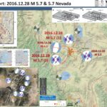
Well, this is an interesting series of earthquakes. They occurred in a region that has not had any earthquakes (given the USGS NEIC database). However, as Jascha Polet pointed out on twitter, there was a swarm to the east in 2011 (here is the University of Nevada Reno Seimological Laboratory page on these 2011 Hawthorne Earthquake Sequence). These two swarms are slightly different in this complicated region of the Pacific-North America plate boundary. A portion of the Pacific-North America plate boundary motion is partitioned along the eastern side of the Sierra Nevada mountains along the Eastern California shear zone, the Walker Lane, and eventually zones like the Mohawk Valley fault zone. Further to the east exists Basin and Range (B&R) extension and along the boundary there is some combination of dextral (right-lateral) shear and B&R extension.

Below I present an interpretive poster for this earthquake series.

I plot the seismicity from the past week, with color representing time and diameter representing magnitude (see legend). I include the active faults from the USGS active fault and fold database. I include moment tensors for the four largest earthquakes in this series.

  • I placed a moment tensor / focal mechanism legend on the poster. There is more material from the USGS web sites about moment tensors and focal mechanisms (the beach ball symbols). Both moment tensors and focal mechanisms are solutions to seismologic data that reveal two possible interpretations for fault orientation and sense of motion. One must use other information, like the regional tectonics, to interpret which of the two possibilities is more likely. The moment tensor shows northeast-southwest compression, perpendicular to the convergence at this plate boundary. Most of the recent seismicity in this region is associated with convergence along the New Britain trench or the South Solomon trench.

At first, I saw the strike-slip moment tensors and thought about the Mina deflection, which is actually further to the south of this swarm. The Mina deflection is an interesting area where the plate boundary motion is diverted to the east along sinistral (left lateral) faults formed by rotating blocks (Lee et al., 2009; Wesnousky et al., 2010, 2012; Rinke et al., 2012; Bormann et al., 2016). There is still debate about how plate motion is accommodated in this region.
What I found interesting is that these 2016 earthquakes do not (at first) appear to fit any existing tectonic model, but are consistent with some faults mapped that may be associated with the 2011 earthquakes. The Wassuk fault to the east accommodates dextral slip associated with the plate boundary (Adams and Sawyer, 1999 (A)). Other faults in the region are characterized a little differently. The mapped faults that probably were activated in 2011 (Adams and Sawyer, 1998) are considered left-lateral and normal. The existing mapped faults to the south of this 2016 swarm are mapped as normal faults based upon offset topography (Adams and Sawyer, 1998 (B)). These unnamed faults west of Aurora Crater, possibly activated today, are classified as younger than 1.6 Ma and have a low slip rate (< 0.2 mm/yr). It is possible that these Aurora Crater faults are more active than 1.6 Ma or that other, more active faults, have not yet been mapped yet. Unfortunately, the M 5.7 probably won't produce surface rupture. What is interesting is that the strike-slip faults in the Mina deflection (MD) to the south are either northwesterly trending dextral or easterly trending sinistral faults. I will discuss this below when I present others' figures. Both interpretations seem possible, but I favor a northeast striking left-lateral interpretation.

    Here are the USGS websites for the larger earthquakes in this 2016 swarm.

  • 2016.12.28 08:22 M 5.7
  • 2016.12.28 08:18 M 5.7
  • 2016.12.28 09:13 M 5.5
  • 2016.12.28 12:18 M 4.1

    I include some inset figures in the poster.

  • In the upper right corner, I include a map that shows the plate boundary scale tectonics for the western US (Nagorsen-Rinke et al., 2012). I placed a yellow star in the general location of the 2016 earthquake series.
  • To the left of this map I include an illustration from Lee et al. (2009) that shows how the faults in the Mina deflection may have formed. Another version of this figure is found in Nagorsen-Rinke et al. (2012). Note how the sinistral faults form as the blocks rotate between faults formed through dextral shear formed by the Pacific-North America plate boundary motion.
  • In the lower right corner I include a smaller scale map that shows the regional scale faulting in the region (Nagorsen-Rinke et al., 2012). I place a yellow star in the location of today’s earthquake swarm.
  • In the upper left corner I include a map from Bormann et al. (2016) that shows tectonic domains as devised by the authors based upon Global Positioning System (GPS) geodetic observations. GPS geodesy is the study of the deformation of Earth’s surface through the use of GPS observations for 3-D positions. I place a red star where today’s earthquakes occurred. Note how these earthquakes are along the boundary of the Mono Basin and Walker Range tectonic domains. There are many short faults in this region forming a complicated tectonic region. The low slip rates for these faults make it difficult to use GPS geodesy to resolve the strain and sense of motion along these faults.
  • Below this map I include the USGS Did You Feel It? maps for the 4 largest earthquakes. These maps show estimates of ground motions that is actually based on real observations as submitted to the USGS website for each of these earthquakes. Note how the M 4.1 was felt in slightly different regions than the other earthquakes. The M 4.1 earthquake was an extensional earthquake, compared to strike-slip for the others. This most likely contributed to these variations in ground motions, in addition to the magnitude differences.
  • In the lower left corner I include a Google Earth map that shows the seismicity from 1900-2016 for earthquakes with magnitudes M ≥ 4.0. I outline the 2011 and 2016 regions of seismicity in dashed white lines. Here is the query that I used to find these earthquakes. I label the major fault zones in this region. Note how the 2011 swarm was mostly extensional, but there were a few strike-slip earthquakes. If these are related to the unnamed faults near Alkali Valley, then they are probably northeast striking sinistral (left-lateral) strike-slip earthquakes.


  • Here are the two figures from Rinke et al. (2012) that show the global and regional tectonics here. I include the figure captions below as blockquotes. The first map shows the plate boundary scale tectonic regions. This is a generalized map (e.g. don’t pay attention to where the San Andreas and Cascadia faults are located). The second map shows the regional fault systems.

  • Simplified tectonic map of the western U.S. Cordillera showing the modern plate boundaries and tectonic provinces. Basin and Range Province is in medium gray; Central Nevada seismic belt (CNSB), eastern California shear zone (ECSZ), Intermountain seismic belt (ISB), and Walker Lane belt (WLB) are in light gray; Mina deflection (MD) is in dark gray.


    Shaded relief map of the WLB and northern part of the ECSZ showing the major Quaternary faults. Solid ball is located on the hanging wall of normal faults; arrow pairs indicate relative motion across strike-slip faults; white dashed box outlines location of Figure 2; light gray shaded areas show the Mina deflection and the Carson domain. BSF—Benton Springs fault; CF—Coaldale fault; DSF—Deep Springs fault; DVFCFLVFZ—Death Valley–Furnace Creek–Fish Lake Valley fault zone; GHF—Gumdrop Hills fault; HLF—Honey Lake fault; HMF—Hunter Mountain fault; MVF—Mohawk Valley fault; OVF— Owens Valley fault; PLF—Pyramid Lake fault; PSF—Petrifi ed Springs fault; QVF—Queen Valley fault; SLF—Stateline fault; SNFFZ—Sierra Nevada frontal fault zone; WMFZ—White Mountains fault zone; WRF—Wassuk Range fault; WSFZ—Warm Springs fault zone.

  • Here is a figure from Wesnousky et al. (2012) where a wax block model is used to illustrate their interpretations of the tectonic deformation along the Walker Lane region. Today’s earthquakes occurred in the basin to the west of the circled number “7.”

  • (Left) Model to visualize accommodation of strain and development of basins in northern Walker lane. The upper is a block of wax has been heated to become ductile and subjected to transtensional right-lateral shear. Ice has been applied to the surface of lower wax block to create brittle upon ductile layer, and then subjected to same shear. The transtensional shear results in a zone of deformation displaying rotation of ‘crustal blocks’, an en echelon arrangement of asymmetric ‘basins,’ observable extension along the axis of shear, and the ability to locally traverse the entire zone of shear without encountering a major fault structure. (Right) Oblique view of study area illustrates the en echelon arrangement and triangular shape of basins nested along the east edge of the Sierra Nevada. Black and colored lines are portions of Walker Lane faults shown in Fig. 1 (Wesnousky et al., 2012)

  • Here are the geodetic observations for each of these blocks along the Walker Lane (Wesnousky et al., 2012). GPS rates are plotted as red vectors. Geologic rates are in the white boxes and are plotted as vectors in black, purple, and blue. Today’s earthquake series happened in the basin where the label “LUCK” is. Note how the GPS site on the northeast side of the basin is moving slightly faster than the GPS site on the western side of the basin. A northwesterly striking right-lateral strike-slip fault could produce this if it ran between these two GPS sites.

  • Physiographic and fault map of area of interest in northern Walker Lane shows major structural basins (numbered), active basin-bounding faults (thick black lines), and geodetic displacement field (red arrows). Shown in white boxes are geologically determined values of fault-normal extension (black-upper text), geodetic estimates of fault-normal extension (magenta-middle text) and geodetic estimates of fault-parallel strike-slip (blue-lower text) rates along each of the basin bounding faults. Two-headed arrows schematically show ranges of same values and correspond in arrangement and color to the values in boxes. The geologically determined extension rate arrows are placed adjacent to the sites of studies except for Lake Tahoe where the estimate is an average value across several submarine faults. Dotted (yellow) lines define paths AB, CD, and EF.

  • This is the tectonic domain figure from Bormann et al. (2016). Some faults have arrows that show their relative sense of motion and blocks have arrows that show their relative sense of rotation. Note the east-west sinistral strike-slip faults that bound the northern and southern boundaries of the blocks in the Mina deflection. Today’s earthquakes happened along the eastern boundary of the Bodie Hills tectonic domain (BH). The BH domain has clockwise rotation like in the Mina deflection. This would place sinistral strain along the southern boundary of the BH domain, creating left-lateral strike-slip faults oriented northeast striking. This is consistent with the sense of motion along the “unnamed faults near Alkali Valley.” If these 2016 earthquakes are associated with these faults, then they are along northeast striking structures and would be left-lateral.

  • Regional map showing the block model boundaries (yellow lines) in relation to the topography and faults of the Central Walker Lane. The Central Walker Lane (region within the dashed black lines) lies between the northeast striking normal faults of the Basin and Range and the Sierra Nevada microplate. Black lines delin-eate major normal faults of the Central Walker Lane, and red lines mark the location of strike slip faults (arrows indicate slip direction). Paleomagnetic observations in-dicate that crustal blocks in the Carson Domain, Bodie Hills, and Mina Deflection accommodate dextral shear through clockwise vertical axis rotations (Cashman and Fontaine, 2000; Petronis et al., 2009; Rood et al., 2011b; Carlson et al., 2013). Orange lines mark the locations of surface rupture that resulted from historic earthquakes in the Central Nevada Seismic Belt. Faults traces are modified from the USGS Qua-ternary Fault and Fold database (U.S. Geological Survey, California Geological Survey, Nevada Bureau of Mines and Geology, 2006). Inset map shows the location of the study area in relation to other elements of the Pacific/North America Plate boundary zone.

  • Here Bormann et al. (2016) present their estimates of rotation and fault slip rates for this region. The caption is below the figure. I place a red star where today’s earthquakes happened. This map helps us visualize an alternate interpretation of these earthquakes. The 2016 swarm is along the eastern boundary of the BH domain, which would suggest a northwest striking dextral (right-lateral) strike slip fault would be involved. Given that the currently mapped faults in this region are northeast striking, I interpret these to be along structures that are also northeast striking. Note how the BH domain is rotating clockwise about 1.75 °/Ma, while the MD is rotating clockwise about 2.75 °/Ma.

  • Block motions, slip rates, and velocity residuals for the best fitting GPS model. (A) Rigid block rotation and translation exaggerated by a factor of 107(representing 10 million years of deformation). Color of block indicates vertical axis rotation rate. (B) Predicted fault slip rates represented by the thickness of black (red) line for dextral (sinistral) strike-slip motion and the length of blue (cyan) bar for fault normal extension (compression).

  • Here is the illustrative model presented by Lee et al. (2009) to explain the faulting in the MD (which may also partially explain the seismicity in this region northeast of the Bodie Hills).

  • Schematic block diagrams illustrating two fault-slip transfer mechanisms between subparallel strike-slip faults proposed for the eastern California shear zone and Walker Lane belt. (A) Displacement transfer model whereby the magnitude of extension along the connecting normal faults is proportional to the amount of strike-slip motion transferred (modified from Oldow et al., 1994). (B) Block rotation model in which clockwise rotation of blocks, bounded by dextral faults, is accommodated by sinistral faults (model of McKenzie and Jackson, 1983, 1986).

  • Here is an updated figure to show how these fault systems may have evolved through time (Nagorsen-Rinke et al., 2012).

  • Block diagrams illustrating models proposed to explain fault slip transfer across the Mina deflection. (A) Displacement transfer model in which normal slip along connecting faults transfers fault slip (modified from Oldow, 1992; Oldow et al., 1994). (B) Transtensional model showing a combination of sinistral and normal slip along connecting faults. (C) Clockwise block rotation model in which sinistral slip along connecting faults, combined with vertical axis rotation of intervening fault blocks, transfers fault slip (modified from McKenzie and Jackson, 1983, 1986). Single-barbed arrows show dextral fault motion across faults of the Eastern California shear zone (ECSZ) and Walker Lane belt (WLB) and sinistral motion along faults in the Mina deflection; half-circle double-barbed arrows indicate clockwise rotating fault blocks; solid ball is located on the hanging wall of normal slip faults; thin short lines indicate slip direction on fault surfaces.

  • Here is the map from the UNR Seismological Laboratory website. This shows the earthquakes recorded during the 2011 swarm along the “unnamed faults along Alakali Valley.” Here is the UNRSL website for this earthquake. I include the UNRSL description of the 2011 Hawthorne Sequence below.

    • Over the past nine weeks 42 earthquakes of Magnitude 3.0 and larger earthquakes (listed below) have been located in a sequence about 12 miles southwest of Hawthorne, Nevada. The first of these occurred on March 15th at 11:14 AM PDT and the latest at 10:23 AM PDT on May 19th. The preliminary magnitude for the largest event is M 4.6.
    • In all, there have been several hundred events of Magnitude 1 and larger; only a small fraction of the entire sequence has been reviewed. There have been 1000’s of smaller magnitude events.
    • The Nevada Seismological Laboratory deployed 3 temporary telemetered instruments in the source area on April 17-19 including a NetQuakes instrument at the Court House in Hawthorne. These temporary telemetered instruments deliver real-time data to the data center in Reno and are configured with 3-channel broadband sensors and 3-channel accelerometers.
  • Here is a map from Nagorsen-Rinke et al. (2012) with regional faults mapped. Note how the sisnistral faults that bound blocks in the Mina deflection are each slightly more counterclockwise rotated with the fault at the base of the southeastern Excelsior Mountains being the most northerly striking of these faults. If this configuration of faulting were in the basin to the NE of the Bodie Hills, it would explain the northeast striking sinistral interpretation for the 2016 series.

  • Shaded relief map of the southern part of the Mina deflection and northern part of the eastern California shear zone showing the major Quaternary faults. Solid black ball is located on the hanging wall of normal faults; arrow pairs indicate relative motion across strike-slip faults. Heavy arrow in northwest corner of map shows the present-day motion of the Sierra Nevada (SN) with respect to North America (NA) (Dixon et al., 2000). Location of the Adobe Hills geologic map shown in Figure 4A is outlined with a dashed line and location of this map is shown in Figure 1. PS—Pizona Springs; CF—Coaldale fault; CSF— Coyote Springs fault; DSF—Deep Springs fault; FLVFZ—Fish Lake Valley fault zone; HCF—Hilton Creek fault; OVF—Owens Valley fault; QVF—Queen Valley fault; RVF— Round Valley fault; WMFZ—White Mountains fault zone.

  • Here is the comparison map for the 2011 and 2016 earthquakes. This is the same data set as presented in the poster above, but I include the 2016 moment tensors here. If the two M 5.7 and one M 5.5 earthquakes are along a NW striking fault, it would be dipping at ~42° and daylight ~4km to the southwest. There is an east-west striking fault mapped at this distance and with this strike immediately to the east of the M 5.7 (2) moment tensor. The strike of this mapped fault is actually more aligned with the moment tensors than the other north striking Aurora Crater faults. What do you think?

References:

  • Adams, K., and Sawyer, T.L., compilers, 1998 (A), Fault number 1299, Unnamed faults near Alkali Valley, in Quaternary fault and fold database of the United States: U.S. Geological Survey website, https://earthquakes.usgs.gov/hazards/qfaults, accessed 12/28/2016 11:51 AM.
  • Adams, K., and Sawyer, T.L., compilers, 1998 (B), Fault number 1298, Unnamed faults west of Aurora Crater, in Quaternary fault and fold database of the United States: U.S. Geological Survey website, https://earthquakes.usgs.gov/hazards/qfaults, accessed 12/28/2016 10:11 AM.
  • Adams, K., and Sawyer, T.L., compilers, 1999, Fault number 1300, Wassuk Range fault zone, in Quaternary fault and fold database of the United States: U.S. Geological Survey website, https://earthquakes.usgs.gov/hazards/qfaults, accessed 12/28/2016 11:52 AM.
  • Bormann, J.M., Hammond, W.C., Kreemer, C., and Blewitt, G., 2016. Accommodation of missing shear strain in the Central Walker Lane, western North America: Constraints from dense GPS measurements in EPSL, v. 440, p. 169-177.
  • Lee, J., Garwood, J., Stockli, D.F., and Gosse, J., 2009. Quaternary faulting in Queen Valley, California-Nevada: Implications for kinematics of fault-slip transfer in the eastern California shear zone Walker Lane belt in GSA Bulletin, v. 121, no. 3/4, p. 599-614.
  • Nagorsen-Rinke, S., Lee, J., and Clavert, A., 2012. Pliocene sinistral slip across the Adobe Hills, eastern California–western Nevada: Kinematics of fault slip transfer across the Mina deflection in Geosphere, v. 9, no. 1, p. 37-53.
  • Stockli, D.F., Dumitru, T.A., McWilliams, M.O., and Farley, K.A., 2003. Cenozoic tectonic evolution of the White Mountains,California and Nevada in GSA Bulletin, v. 115, no. 7, p/ 788-816.
  • Wesnouskky, S.G., Bormann, J.M., Kreemer, C., Hammond, W.C., and Brune, J.N., 2012. Neotectonics, geodesy, and seismic hazard in the Northern Walker Lane of Western North America: Thirty kilometers of crustal shear and no strike-slip? in EPSL, v. 329-330, p. 133-140.

Earthquake Anniversary: Sumatra-Andaman 2004 M 9.2 & 2005 M 8.6

On 26 December 2004 there was an earthquake with a magnitude of M 9.2 along the Sumatra-Andaman subduction zone (SASZ). This earthquake is the third largest earthquake ever recorded by modern seismometers and ruptured nearly 2,000 km of the megathrust fault offshore of Sumatra, the Andaman Isles, and the Nicobar Isles. (The 22 may 2960 Chile M 9.5 and 27 March 1964 M 9.2 Good Friday earthquake in Alaska are the first and second largest.) This 2004 M 9.2 earthquake triggered submarine landslides and deformed the seafloor to generate a trans-oceanic tsunami that killed almost a quarter of a million people. A few months later, on 28 March 2005, there was another megathrust earthquake, further to the south, with a magnitude of M 8.6. The M 8.6 earthquake ruptured in a region of the megathrust that had an increase in coulomb stress imparted to it by the M 9.2 earthquake to the north. The increase in stress is small, so for the stress increase to be able to trigger an earthquake, the fault must be within a margin of critical stress prior to the first earthquake in order to be triggered.
In prior years, I have written some material about the 2004 earthquake, including some observations made by others. Today I prepared an interpretive poster for the 2004 and 2005 SASZ earthquakes (while waking up at my mom’s house, where I was for the holiday; I was driving home to Arcata in 2004 when I heard about the SASZ earthquake.).
I updated this page for the 2017 anniversary of this 2004 earthquake in some places.

    Here are the USGS websites for these two SASZ earthquakes.

  • 2004.12.26 M 9.2
  • 2005.03.28 M 8.6

    Here is a summary page from IRIS.

  • 2004.12.26 M 9.2

Below is my interpretive poster for this earthquake.

I plot the seismicity from the past month, with color representing depth and diameter representing magnitude (see legend). I also include the region of the fault slip solution as modeled by the USGS (slightly transparent blue polygons). Note how the 2005 earthquake slips along a section of the fault that is further down-dip compared to the 2004 earthquake. This probably owes to the smaller tsunami triggered by the 2005 earthquake (and the smaller turbidite; Patton et al., 2015).

  • I placed a moment tensor / focal mechanism legend on the poster. There is more material from the USGS web sites about moment tensors and focal mechanisms (the beach ball symbols). Both moment tensors and focal mechanisms are solutions to seismologic data that reveal two possible interpretations for fault orientation and sense of motion. One must use other information, like the regional tectonics, to interpret which of the two possibilities is more likely. The moment tensor shows northeast-southwest compression, perpendicular to the convergence at this plate boundary. Most of the recent seismicity in this region is associated with convergence along the New Britain trench or the South Solomon trench.
  • I also include the shaking intensity contours on the map. These use the Modified Mercalli Intensity Scale (MMI; see the legend on the map). This is based upon a computer model estimate of ground motions, different from the “Did You Feel It?” estimate of ground motions that is actually based on real observations. The MMI is a qualitative measure of shaking intensity. More on the MMI scale can be found here and here. This is based upon a computer model estimate of ground motions, different from the “Did You Feel It?” estimate of ground motions that is actually based on real observations.
  • I include the MMI contours for both 2004 and 2005 earthquakes.
  • I include the slab contours plotted (Hayes et al., 2012), which are contours that represent the depth to the subduction zone fault. These are mostly based upon seismicity. The depths of the earthquakes have considerable error and do not all occur along the subduction zone faults, so these slab contours are simply the best estimate for the location of the fault. The hypocentral depth plots this close to the location of the fault as mapped by Hayes et al. (2012).

    I include some inset figures in the poster.

  • In the upper left corner, I include a map that shows the extent of historic earthquakes along the SASZ offshore of Sumatra. This map is a culmination of a variety of papers (summarized and presented in Patton et al., 2015).
  • In the upper right corner I include a figure that is presented by Chlieh et al. (2007). These figures show model results from several models. Each model is represented by a map showing the amount that the fault slipped in particular regions. I present this figure below.
  • In the lower right corner I present a figure from Prawirodirdjo et al. (2010). This figure shows the coseismic vertical and horizontal motions from the 2004 and 2005 earthquakes as measured at GPS sites.
  • In the lower left corner are the MMI intensity maps for the two SASZ earthquakes. Note these are at different map scales. I also include the MMI attenuation curves for these earthquakes below the maps. These plots show the reported MMI intensity data as they relate to two plots of modeled estimates (the orange and green lines). These green dots are from the USGS “Did You Feel It?” reports compared to the estimates of ground shaking from Ground Motion Prediction Equation (GMPE) estimates. GMPE are empirical relations between earthquakes and recorded seismologic observations from those earthquakes, largely controlled by distance to the fault, ray path (direction and material properties), and site effects (the local geology). When seismic waves propagate through sediment, the magnitude of the ground motions increases in comparison to when seismic waves propagate through bedrock. The orange line is a regression of data for the central and eastern US and the green line is a regression through data from the western US.


  • Here is the USGS poster for this earthquake. These results were put out very soon after the earthquake and later reports made more refined analyses. For example, there are over a dozen earthquake slip models for this earthquake, most all are better than this initial USGS version.

  • Here are the map and attenuation plots as a single figure.

  • Here is a figure that shows the wave height observations from satellites that happened to be passing over the Indian Ocean as the tsunami crossed towards India and Sri Lanka (Shearer and Burgman 2010).

  • This figure from Meltzner et al. (2010) shows measurements of vertical deformation collected from coral microatolls (which are sensitive to the tides, basically, they cannot survive above a certain level of tidal elevation. Read his and related papers to learn more about this method.). These are observations that are independent of GPS data.

  • Here is the source time function from Ishi et al. (2005). Note the similarity between this plot and the above one from Chlieh et al. (2007). These results are more comparable that the slip models we saw earlier.

  • This is from Subarya et al. (2006), an earlier plot, but still similar to Chlieh et al. (2007) and Ishii et al. (2007).

  • This is another estimate published also in 2006 (Tolstoy and Bohnenstiehl, 2006), again showing similarities with the other plots (though this is the most different). There are a number of other examples as well (e.g. Okal).

  • UPDATE 2017: Below is a plot of the seismographs from a global data set, prepared by IRIS and others.

  • This record section plot displays vertical displacements of the Earth’s surface recorded by seismometers plotted with time (since the earthquake initiation) on the horizontal axis, and vertical displacements of the Earth on the vertical axis (note the 1 cm scale bar at the bottom for scale). The traces are arranged by distance from the epicenter in degrees. The earliest, lower amplitude, signal is that of the compressional (P) wave, which takes about 22 minutes to reach the other side of the planet (the antipode). The largest amplitude signals are seismic surface waves that reach the antipode after about 100 minutes. The surface waves can be clearly seen to reinforce near the antipode (with the closest seismic stations in Ecuador), and to subsequently circle the planet to return to the epicentral region after about 200 minutes. A major aftershock (magnitude 7.1) can be seen at the closest stations starting just after the 200 minute mark (note the relative size of this aftershock, which would be considered a major earthquake under ordinary circumstances, compared to the mainshock).

  • UPDATE 2017:This is a video showing a visualization of the seismic waves transmitted from the 2004 SASZ earthquake from IRIS and others.
  • This movie illustrates simulation of seismic wave propagation generated by Dec. 26 Sumatra earthquake. Colors indicate amplitude of vertical displacement at the surface of the Earth. Red is upward and blue is downward. Total duration of this simulation is 20 minutes. Source model we used is that of Chen Ji of Caltech. Simulation was performed by using the Earth Simulator of JAMSTEC.

  • These next two figures from Singh et al. (2008 ) show a map and cross section at the location of the earthquake. The 2004 SASZ earthquake ruptured very deep in a location previously thought to not harbor strain to be accumulated and released during an earthquake.

  • In 2007 Dr. Chris Goldfinger and myself led a coring expedition in this region within Indonesian EEZ and international waters offshore of Sumatra. Our goal was to evaluate the sedimentary record of earthquakes in the form of submarine landslide deposits (called turbidites). We collected over 100 sediment cores and have prepared several papers documenting some of our results (Patton et al., 2013, 2015).
  • I will be preparing a website that documents this 2007 cruise aboard the R/V Roger Revelle. Here is the website. On this website, I provide a link to my research cruise blog, where I documented my cruise in real time. This is the first blog post for the RR0705 cruise.
  • Below is a figure where I present evidence for a sedimentary deposit from the 2004 SASZ earthquake (Patton et al., 2015). Sumner et al. (2013) also present sedimentary evidence for the 2004 earthquake. Especially convincing because they observed computer paper within the turbidite! I include a figure caption below the image in blockquote.

  • The uppermost (2004?) turbidite from cores 96PC and 96TC, plotted as a composite core. A. From left to right: mean particle size, point magnetic susceptibility, CT density, gamma density, turbidite classification, RGB imagery, CT imagery, turbidite structure classification division, depth (cm), turbidite structure (lithologic log), texture, and the lithologic notes are plotted vs. depth. Geophysical logs symbolized as in Figure 2. B. Detailed turbidite structure based on CT imagery. From left to right: i. CT imagery uninterpreted, ii. CT imagery interpreted, iii. Turbidite structure interpretation, iv. Turbidite structure division classification, and v. turbidite structure description. C. Results from smear slide based vertical biostratigraphic transects for core 96PC. Percent biogenic and percent lithologic are plotted vs. depth in m. D. The mean, minimum, and maximum particle size distribution for sediments collected within the uppermost turbidite (in purple) and within hemipelagic sediments underlying the uppermost turbidite (in green) are plotted. These are compared with the combined distributions (in blue).

  • Here is the cross section showing where the earthquake hypocenter is compared to where we think the mantle exists. We have not been here, so nobody actually knows… These interpretations are based on industry deep seismic data (Singh et al., 2008 ).

  • Here is the historic rupture map again. I include a figure caption below that I wrote as blockquote.

  • India-Australia plate subducts northeastwardly beneath the Sunda plate (part of Eurasia) at modern rates (GPS velocities are based on regional modeling of Bock et al, 2003 as plotted in Subarya et al., 2006). Historic earthquake ruptures (Bilham, 2005; Malik et al., 2011) are plotted in orange. 2004 earthquake and 2005 earthquake 5 meter slip contours are plotted in orange and green respectively (Chlieh et al., 2007, 2008). Bengal and Nicobar fans cover structures of the India-Australia plate in the northern part of the map. RR0705 cores are plotted as light blue. SRTM bathymetry and topography is in shaded relief and colored vs. depth/elevation (Smith and Sandwell, 1997).

  • Here is a cross section showing the differences of vertical deformation between the coseismic (during the earthquake) and interseismic (between earthquakes). This diagram was created to explain the deformation observed during the Good Friday Alaska earthquake, but these observations are observed during earthquakes at subduction zones globally.

  • This figure, from Atwater et al. (2005) shows the earthquake deformation cycle and includes the aspect that the uplift deformation of the seafloor can cause a tsunami.

  • Here is the inset figure from Chlieh et al. (2007). I include a figure caption below in blockquote.

  • Observed (black) and Predicted (red) vertical displacements associated to model Ammon-III [Ammon et al. 2005] (A, See figure 5 in the main text), model G-M9.12 (B, figure 6), model G-M9.22 (C, figure 7) and our preferred coseismic model G-M9.15 (D, figure 9 in the main text).

    Here are some pages where I present information about these SASZ earthquakes.

  • 2014.12.21 General Overview of the regional tectonics and SASZ earthquakes
  • 2014.12.25 Sumatra-Andaman subduction zone 2014/12/26: Slip, Deformation, and Energy

    Additional Static Stress Triggering!

  • The 2004/2005 SASZ earthquakes also tended to load strain in the crust in different locations. On 2012.04.11 there was a series of strike-slip earthquakes in the India plate crust to the west of the 2004/2005 earthquakes. The two largest magnitudes for these earthquakes were M 8.6 and M 8.2. The M 8.6 is the largest strike-slip earthquake ever recorded.
  • On 2016.03.22 there was another large strike-slip earthquake in the India-Australia plate. This is probably related to this entire suite of subduction zone and intraplate earthquakes. I presented an interpretive poster about this M 7.8 earthquake here. Below is my interpretive poster for the M 7.8 earthquake. Here is the USGS website for this earthquake.
  • I include a map in the upper right corner that shows the historic earthquake rupture areas.

  • Here is a poster that shows some earthquakes in the Andaman Sea. This is from my earthquake report from 2015.11.08.

  • This map shows the fracture zones in the India-Australia plate.

  • UPDATE 2017: Below is a video from IRIS that discusses the 2004 and 2012 earthquakes.
  • Data released in the Sept 2012 Nature journal yielded new information about the 2012 Sumatra earthquake. Surprising elements of this earthquake include, that it was both the largest intra-plate earthquake and the largest strike-slip earthquake ever recorded, plus the 10th largest earthquake of any kind ever recorded. Not to mention the most complex.
    In 2004 a Magnitude 9.1 interplate subduction earthquake triggered a tsunami that killed over 230,000 people. Yet a nearby magnitude 8.7 intraplate earthquake in 2012, caused little damage and generated minimal ocean waves. Although the earthquakes appeared similar in magnitude and were close in proximity, they were caused by different tectonic processes related to the greater Indo Australian plate.
    This animation describes the different tectonic settings of the two plates, and how the Indo-Australian plate seems destined to become two distinct tectonic plates: the Indian and the Australian plates.
    Yue, Lay, Koper Nature article:
    https://www.nature.com/articles/nature11492
    Animation by Jenda Johnson, Earth Sciences Animated

References:

  • Atwater, B.F., Yamaguchi, D.K., Bondevik, S., Barnhardt, W.A., Amidon, L.J., Benson, B.E., Skjerdal, G., Shulene, J.A., and Nanalyama ,F., 2001. Rapid resetting of an estuarine recorder of the 1964 Alaska earthquake in Geology, v. 113, no. 9, p. 1193-1204.
  • Bilham, R., 2005. Partial and Complete Rupture of the Indo-Andaman Plate Boundary 1847 – 2004: Seismological Research Letters, v. 76, p. 299-311.
  • Bock, Y., Prawirodirdjo, L., Genrich, J.F., Stevens, C.W., McCaffrey, R., Subarya, C., Puntodewo, S.S.O., Calais, E., 2003. Crustal motion in Indonesia from Global Positioning System measurements: Journal of Geophysical Research, v. 108, no. B8, 2367, doi: 10.1029/2001JB000324.
  • Briggs, R.W., Sieh, K., Meltzner, A.J., Natawidjaja, D., Galetzka, J., Suwargadi, B., Hsu, Y.-j., Simons, M., Hananto, N., Suprihanto, I., Prayudi, D., Avouac, J.-P., Prawirodirdjo, L., Bock, Y., 2006. Deformation and Slip Along the Sunda Megathrust in the Great 2005 Nias-Simeulue Earthquake: Science, v. 311, p. 1,897-1,901.
  • Chlieh, M., Avouac, J.-P., Hjorleifsdottir, V., Song, T.-R.A., Ji, C., Sieh, K., Sladen, A., Hebert, H., Prawirodirdjo, L., Bock, Y., Galetzka, J., 2007. Coseismic Slip and Afterslip of the Great (Mw 9.15) Sumatra-Andaman Earthquake of 2004: Bulletin of the Seismological Society of America, v. 97, no. 1A, p. S152-S173, doi: 10.1785/0120050631.
  • Chlieh, M., Avouac, J.P., Sieh, K., Natawidjaja, D.H., Galetzka, J., 2008. Heterogeneous coupling of the Sumatran megathrust constrained by geodetic and paleogeodetic measurements: Journal of Geophysical Research, v. 113, B05305, doi: 10.1029/2007JB004981.
  • Hayes, G.P., Wald, D.J., and Johnson, R.L., 2012. Slab1.0: A three-dimensional model of global subduction zone geometries in, J. Geophys. Res., 117, B01302, doi:10.1029/2011JB008524
  • Ishii, M., Shearer, P.M., Houston, H., Vidale, J.E., 2005. Extent, duration and speed of the 2004 Sumatra-Andaman earthquake imaged by the Hi-Net array. Nature 435, 933.
  • Malik, J.N., Shishikura, M., Echigo, T., Ikeda, Y., Satake, K., Kayanne, H., Sawai, Y., Murty, C.V.R., Dikshit, D., 2011. Geologic evidence for two pre-2004 earthquakes during recent centuries near Port Blair, South Andaman Island, India: Geology, v. 39, p. 559-562.
  • Meltzner, A.J., Sieh, K., Chiang, H., Shen, C., Suwargadi, B.W., Natawidjaja, D.H., Philobosian, B., Briggs, R.W., Galetzka, J., 2010. Coral evidence for earthquake recurrence and an A.D. 1390–1455 cluster at the south end of the 2004 Aceh–Andaman rupture. Journal of Geophysical Research 115, 1-46.
  • Patton, J. R., Goldfinger, C., Morey, A. E., Romsos, C., Black, B., Djadjadihardja, Y., Udrekh, 2013, Seismoturbidite Record as Preserved at Core Sites at the Cascadia and Sumatra‐Andaman Subduction Zones: : The Offshore Search of Large Holocene Earthquakes: Obergurgl, Austria, Natural Hazards and Earth System Sciences, 13, p. 833‐867
  • Patton, J. R., Goldfinger, C., Morey, A. E., Ikehara, K., Romsos, C., Stoner, J., Djadjadihardja, Y., Udrekh, Ardhyastuti, S., Gaffar, E.Z., and Viscaino, A. A 6500 year earthquake history in the region of the 2004 Sumatra‐Andaman subduction zone Earthquake, Geosphere, vol. 11, no. 6, p. 1‐62, doi:10.1130/GES01066.1
  • Plafker, G., 1969. Tectonics of the March 27, 1964 Alaska earthquake: U.S. Geological Survey Professional Paper 543–I, 74 p., 2 sheets, scales 1:2,000,000 and 1:500,000, http://pubs.usgs.gov/pp/0543i/.
  • Prawirodirdjo, P., McCaffrey,R., Chadwell, D., Bock, Y, and Subarya, C., 2010. Geodetic observations of an earthquake cycle at the Sumatra subduction zone: Role of interseismic strain segmentation, JOURNAL OF GEOPHYSICAL RESEARCH, v. 115, B03414, doi:10.1029/2008JB006139
  • Rajendran, C.P., Rajendran, K., Anu, R., Earnest, A., Machado, T., Mohan, P.M., Freymueller, J., 2007. Crustal Deformation and Seismic History Associated with the 2004 Indian Ocean Earthquake: A Perspective from the Andaman–Nicobar Islands: Bulletin of The Seismological Society of America, v. 97, S174-S191, doi: 10.1785/0120050630.
  • Shearer, P., and Burgmann, R., 2010. Lessons Learned from the 2004 Sumatra-Andaman Megathrust Rupture, Annu. Rev. Earth Planet. Sci. v. 38, pp. 103–31
  • Singh, S.C., Carton, H.L., Tapponnier, P, Hananto, N.D., Chauhan, A.P.S., Hartoyo, D., Bayly, M., Moeljopranoto, S., Bunting, T., Christie, P., Lubis, H., and Martin, J., 2008. Seismic evidence for broken oceanic crust in the 2004 Sumatra earthquake epicentral region, Nature Geoscience, v. 1, pp. 5.
  • Smith, W.H.F., Sandwell, D.T., 1997. Global seafloor topography from satellite altimetry and ship depth soundings: Science, v. 277, p. 1,957-1,962.
  • Sumner, E., Siti, M., McNeil, L.C., Talling, P.J., Henstock, T., Wynn, R., Djadjadihardja, Y., Permana, H., 2013. Can turbidites be used to reconstruct a paleoearthquake record for the central Sumatran margin?: Geology, v. 41, p. 763-766.
  • Subarya, C., Chlieh, M., Prawirodirdjo, L., Avouac, J., Bock, Y., Sieh, K., Meltzner, A.J., Natawidjaja, D.H., McCaffrey, R., 2006. Plate-boundary deformation associated with the great Sumatra–Andaman earthquake: Nature, v. 440, p. 46-51.
  • Tolstoy, M., Bohnenstiehl, D.R., 2006. Hydroacoustic contributions to understanding the December 26th 2004 great Sumatra–Andaman Earthquake. Survey of Geophysics 27, 633-646.
  • Yue, H., Lay, T., and Koper, K.D., 2012. En échelon and orthogonal fault ruptures of the 11 April 2012 great intraplate earthquakes. in Nature, v. 490, p. 245-249, doi:10.1038/nature11492

Earthquake Report: Chile!

Last night we had a large earthquake in the southern region of the 1960 M 9.5 Valdivia earthquake. Below are some USGS websites for the three large earthquakes for this region that I mention in my interpretive poster. Based on the hypocentral depth of ~35 km and the slab contours from Hayes et al. (2012), this appears to be a subduction zone interface earthquake. The epicenter plots between the 20 and 40 km slab contours.

Below is my interpretive poster for this earthquake.

I plot the seismicity from the past month, with color representing depth and diameter representing magnitude (see legend).

  • I placed a moment tensor / focal mechanism legend on the poster. There is more material from the USGS web sites about moment tensors and focal mechanisms (the beach ball symbols). Both moment tensors and focal mechanisms are solutions to seismologic data that reveal two possible interpretations for fault orientation and sense of motion. One must use other information, like the regional tectonics, to interpret which of the two possibilities is more likely. The moment tensor shows northeast-southwest compression, perpendicular to the convergence at this plate boundary. Most of the recent seismicity in this region is associated with convergence along the New Britain trench or the South Solomon trench.
  • I also include the shaking intensity contours on the map. These use the Modified Mercalli Intensity Scale (MMI; see the legend on the map). This is based upon a computer model estimate of ground motions, different from the “Did You Feel It?” estimate of ground motions that is actually based on real observations. The MMI is a qualitative measure of shaking intensity. More on the MMI scale can be found here and here. This is based upon a computer model estimate of ground motions, different from the “Did You Feel It?” estimate of ground motions that is actually based on real observations.
  • I include the slab contours plotted (Hayes et al., 2012), which are contours that represent the depth to the subduction zone fault. These are mostly based upon seismicity. The depths of the earthquakes have considerable error and do not all occur along the subduction zone faults, so these slab contours are simply the best estimate for the location of the fault. The hypocentral depth plots this close to the location of the fault as mapped by Hayes et al. (2012).
  • I also include the latitudinal ranges of historic earthquakes in this region (labeled in green).

    I include some inset figures in the poster.

  • In the upper left corner, I include a time-space diagram from Moernaut et al. (2010).
  • To the right of that space time figure is a plot showing the tsunami recorded at a tide gage 30-40 km to the south of the epicenter. This comes from the Intergovernmental Oceanographic Commission here. Here is the NWS National Tsunami Warning Center tsunami announcement.
  • In the upper right corner I include an inset map from the USGS Seismicity History poster for this region (Rhea et al., 2010). There is one seismicity cross section with its locations plotted on the map. The USGS plot these hypocenters along this cross section and I include that below (with the legend).
  • In the lower left corner are the MMI intensity maps for the three earthquakes listed above: 1960 M 9.5, 2010 M 8.8, and 2016 M 7.6. Note these are at different map scales.


  • This map shows the MMI contours for the 1960 and 2010 earthquakes in addition to this 2016 earthquake. This helps us visualize the spatial extent for these earthquakes with a large range of magnitudes. Recall that an M 9.5 earthquake releases about 32 times the energy that an M 8.5 earthquake releases. Note how the 1960 and 2010 earthquakes span a region between the Juan Fernandez fracture zone and where the Chile Rise intersects the trench, where the 4 fracture zones (Guamblin, Darwin, Taitao, and Tres Montes) intersect the trench.


  • Here is the USGS fault slip model. Note the short rupture length of this earthquake, proportional to the magnitude.

  • Below are some figures from Moreno et al. (2011) that show estimates of locking along the plate interface in this region. I include the figure captions as blockquote.
  • The first figure shows how the region of today’s earthquake is in an area of higher locking.

  • a) Optimal distribution of locking rate in the plate interface. Predicted interseismic velocities and GPS vectors corrected by the postseismic signals are shown by green and blue arrows, respectively. b) Tradeoff curve for a broad range of the smoothing parameter (β). The optimal value for β is 0.0095 located at the inflection of the curve.

  • This second figure shows the moment released during historic earthquakes and the moment accumulated due to seismogenic locking along the megathrust.

  • a) Latitudinal distribution of the coseismic moment (Mc) released by the 1960 Valdivia (Moreno et al., 2009) (red line) and 2010 Maule (Tong et al., 2010) (blue line) earthquakes, and of accumulated deficit of moment (Md) due to interseismic locking of the plate interface 50 (orange line) and 300 (gray line) years after the 1960 earthquake, respectively. The range of errors of the Md rate is depicted by dashed lines. High rate of Md was found in the earthquake rupture boundary, where slip deficit accumulated since 1835 seems to be not completely released by the 2010 Maule earthquake. b) Schematic map showing the deformation processes that control the observed deformation in the southern Andes and the similarity between coseismic and locking patches. Blue and red contours denote the coseismic slip for the 2010 Maule (Tong et al., 2010) and 1960 Valdivia (Moreno et al., 2009) earthquakes, respectively. Patches with locking degree over 0.75 are shown by brown shaded areas. The 1960 earthquake (red star) nucleated in the segment boundary, area that appears to be highly locked at present. The 2011 Mw 7.1 aftershock (gray) may indicate that stress has been transmitted to the southern limit of the Arauco peninsula.

  • Here is the space-time diagram from Moernaut et al., 2010. I include their figure caption below in blockquote.

  • Fig.: Setting and historical earthquakes in South-Central Chile. Data derived from Barrientos (2007); Campos et al. (2002); Melnick et al.(2009)

  • Here is the cross section of the subduction zone just to the south of this Sept/Nov 2015 swarm (Melnick et al., 2006). Below I include the text from the Melnick et al. (2006) figure caption as block text.

  • (A) Seismotectonic segments, rupture zones of historical subduction earthquakes, and main tectonic features of the south-central Andean convergent margin. Earthquakes were compiled from Lomnitz (1970, 2004), Kelleher (1972), Comte et al. (1986), Cifuentes (1989), Beck et al. (1998 ), and Campos et al. (2002). Nazca plate and trench are from Bangs and Cande (1997) and Tebbens and Cande (1997). Maximum extension of glaciers is from Rabassa and Clapperton (1990). F.Z.—fracture zone. (B) Regional morphotectonic units, Quaternary faults, and location of the study area. Trench and slope have been interpreted from multibeam bathymetry and seismic-reflection profiles (Reichert et al., 2002). (C) Profile of the offshore Chile margin at ~37°S, indicated by thick stippled line on the map and based on seismic-reflection profiles SO161-24 and ENAP-017. Integrated Seismological experiment in the Southern Andes (ISSA) local network seismicity (Bohm et al., 2002) is shown by dots; focal mechanism is from Bruhn (2003). Updip limit of seismogenic coupling zone from heat-fl ow measurements (Grevemeyer et al., 2003). Basal accretion of trench sediments from sandbox models (Lohrmann, 2002; Glodny et al., 2005). Convergence parameters from Somoza (1998 ).

  • In September through November of 2015, there was a M 8.3 earthquake further to the north. Below is my interpretive poster for that earthquake and here is my report, where I discuss the relations between the 2010, 2015, and other historic earthquakes in this region. Here is my report from September.

  • Here is a space time diagram from Beck et al. (1998 ). The 2015 earthquake occurs in the region of the 1943 and 1880 earthquakes. I updated this figure to show the latitudinal extent of the 2010 and 2015 earthquakes.

References:

Earthquake Report: Bougainville!

Early this morning my time there was a large earthquake along the San Cristobal Trench, a segment of a convergent plate boundary formed by the subduction of the Solomon Sea plate eastwards beneath the Pacific plate. There was an M 6.1 earthquake in the slip patch region about a week ago that may have imparted stress across the fault in this region. The M 6.1 earthquake was very deep, as is this one. The M 6.1 appears to have been deeper than the megathrust, though the M 7.9 is much closer to the Hayes et al. (2012) fault. It seems possible that the M 6.1 loaded the fault and led to the M 7.9. Someone would need to conduct some coulomb static stress modeling to test this hypothesis. However, it would only be a model result and would likely have an unequivocal result (i.e. we still would not “know” if these earthquakes were related. after all, there has not been a movie about this. heheh).
I also include the swarm that happened about a week ago further to the south, along the South Solomon Trench. There was an M 7.8 earthquake there. Here is my Earthquake Report for this earthquake.

Below is my interpretive poster for this earthquake.

I plot the seismicity from the past month, with color representing depth and diameter representing magnitude (see legend).

  • I placed a moment tensor / focal mechanism legend on the poster. There is more material from the USGS web sites about moment tensors and focal mechanisms (the beach ball symbols). Both moment tensors and focal mechanisms are solutions to seismologic data that reveal two possible interpretations for fault orientation and sense of motion. One must use other information, like the regional tectonics, to interpret which of the two possibilities is more likely. The moment tensor shows northeast-southwest compression, perpendicular to the convergence at this plate boundary. Most of the recent seismicity in this region is associated with convergence along the New Britain trench or the South Solomon trench.
  • I also include the shaking intensity contours on the map. These use the Modified Mercalli Intensity Scale (MMI; see the legend on the map). This is based upon a computer model estimate of ground motions, different from the “Did You Feel It?” estimate of ground motions that is actually based on real observations. The MMI is a qualitative measure of shaking intensity. More on the MMI scale can be found here and here. This is based upon a computer model estimate of ground motions, different from the “Did You Feel It?” estimate of ground motions that is actually based on real observations.
  • I include the slab contours plotted (Hayes et al., 2012), which are contours that represent the depth to the subduction zone fault. These are mostly based upon seismicity. The depths of the earthquakes have considerable error and do not all occur along the subduction zone faults, so these slab contours are simply the best estimate for the location of the fault. The hypocentral depth plots this close to the location of the fault as mapped by Hayes et al. (2012).
  • Here are the USGS web pages for the larger magnitude earthquakes. The earthquakes with plotted moment tensors are in bold. I include a link for the earthquake that happened further along this plate boundary, near the Solomon Islands. Here is a Google Earth kml file that has the earthquakes plotted in the map below.
  • I include some inset figures.

  • In the lower left corner is a generalized tectonic map of the region from Holm et al., 2015. This map shows the major plate boundary faults including the New Britain trench (NBT), one of the main culprits for recent seismicity of this region.
  • In the lower right corner is the USGS fault plane solution plotted in place on a map. This figure shows their model results with color representing the spatial variation in earthquake fault slip for this M 7.8 earthquake. This model is calibrated using seismologic observations.
  • In the upper left corner a figure from Oregon State University, which are based upon Hamilton (1979). “Tectonic microplates of the Melanesian region. Arrows show net plate motion relative to the Australian Plate.” This is from Johnson, 1976. There is a plate tectonic map and a cross section showing the subduction of the Solomon Sea plate.
  • In the upper right corner is a figure from Baldwin et al. (2012). This figure shows a series of cross sections along this convergent plate boundary from the Solomon Islands in the east to Papua New Guinea in the west. Cross section ‘C’ is the most representative for the earthquake today. I present the map and this figure again below, with their original captions.


  • There have been several observations of tsunami in the region. The likelihood for a trans Pacific tsunami as reported by the Pacific Tsunami Warning Center has passed.

  • In earlier earthquake reports, I discussed seismicity from 2000-2015 here. The seismicity on the west of this region appears aligned with north-south shortening along the New Britain trench, while seismicity on the east of this region appears aligned with more east-west shortening. Here is a map that I put together where I show these two tectonic domains with the seismicity from this time period (today’s earthquakes are not plotted on this map, but one may see where they might plot).

  • Here is the generalized tectonic map of the region from Holm et al., 2015. I include the figure caption below as a blockquote.

  • Tectonic setting and mineral deposits of eastern Papua New Guinea and Solomon Islands. The modern arc setting related to formation of the mineral deposits comprises, from west to east, the West Bismarck arc, the New Britain arc, the Tabar-Lihir-Tanga-Feni Chain and the Solomon arc, associated with north-dipping subduction/underthrusting at the Ramu-Markham fault zone, New Britain trench and San Cristobal trench respectively. Arrows denote plate motion direction of the Australian and Pacific plates. Filled triangles denote active subduction. Outlined triangles denote slow or extinct subduction. NBP: North Bismarck plate; SBP: South Bismarck plate; AT: Adelbert Terrane; FT: Finisterre Terrane; RMF: Ramu-Markham fault zone; NBT: New Britain trench.

  • Here is the slab interpretation for the New Britain region from Holm and Richards, 2013. Note the tear in the slab where the New Britain and South Solomon trenches intersect. This feeds into the tectonic domains discussed in my map above and also here. I include the figure caption below as a blockquote.

  • 3-D model of the Solomon slab comprising the subducted Solomon Sea plate, and associated crust of the Woodlark Basin and Australian plate subducted at the New Britain and San Cristobal trenches. Depth is in kilometres; the top surface of the slab is contoured at 20 km intervals from the Earth’s surface (black) to termination of slabrelated seismicity at approximately 550 km depth (light brown). Red line indicates the locations of the Ramu-Markham Fault (RMF)–New Britain trench (NBT)–San Cristobal trench (SCT); other major structures are removed for clarity; NB, New Britain; NI, New Ireland; SI, Solomon Islands; SS, Solomon Sea; TLTF, Tabar–Lihir–Tanga–Feni arc. See text for details.

  • This map shows plate velocities and euler poles for different blocks. Note the counterclockwise motion of the plate that underlies the Solomon Sea (Baldwin et al., 2012). I include the figure caption below as a blockquote.

  • Tectonic maps of the New Guinea region. (a) Seismicity, volcanoes, and plate motion vectors. Plate motion vectors relative to the Australian plate are surface velocity models based on GPS data, fault slip rates, and earthquake focal mechanisms (UNAVCO, http://jules.unavco.org/Voyager/Earth). Earthquake data are sourced from the International Seismological Center EHB Bulletin (http://www.isc.ac.uk); data represent events from January 1994 through January 2009 with constrained focal depths. Background image is generated from http://www.geomapapp.org. Abbreviations: AB, Arafura Basin; AT, Aure Trough; AyT, Ayu Trough; BA, Banda arc; BSSL, Bismarck Sea seismic lineation; BH, Bird’s Head; BT, Banda Trench; BTFZ, Bewani-Torricelli fault zone; DD, Dayman Dome; DEI, D’Entrecasteaux Islands; FP, Fly Platform; GOP, Gulf of Papua; HP, Huon peninsula; LA, Louisiade Archipelago; LFZ, Lowlands fault zone; MaT, Manus Trench; ML, Mt. Lamington; MT, Mt. Trafalgar; MuT, Mussau Trough; MV, Mt. Victory; MTB, Mamberamo thrust belt; MVF, Managalase Plateau volcanic field; NBT, New Britain Trench; NBA, New Britain arc; NF, Nubara fault; NGT, New Guinea Trench; OJP, Ontong Java Plateau; OSF, Owen Stanley fault zone; PFTB, Papuan fold-and-thrust belt; PP, Papuan peninsula; PRi, Pocklington Rise; PT, Pocklington Trough; RMF, Ramu-Markham fault; SST, South Solomons Trench; SA, Solomon arc; SFZ, Sorong fault zone; ST, Seram Trench; TFZ, Tarera-Aiduna fault zone; TJ, AUS-WDKPAC triple junction; TL, Tasman line; TT, Trobriand Trough;WD, Weber Deep;WB, Woodlark Basin;WFTB, Western (Irian) fold-and-thrust belt; WR,Woodlark Rift; WRi, Woodlark Rise; WTB, Weyland thrust; YFZ, Yapen fault zone.White box indicates the location shown in Figure 3. (b) Map of plates, microplates, and tectonic blocks and elements of the New Guinea region. Tectonic elements modified after Hill & Hall (2003). Abbreviations: ADB, Adelbert block; AOB, April ultramafics; AUS, Australian plate; BHB, Bird’s Head block; CM, Cyclops Mountains; CWB, Cendrawasih block; CAR, Caroline microplate; EMD, Ertsberg Mining District; FA, Finisterre arc; IOB, Irian ophiolite belt; KBB, Kubor & Bena blocks (including Bena Bena terrane); LFTB, Lengguru fold-and-thrust belt; MA, Mapenduma anticline; MB, Mamberamo Basin block; MO, Marum ophiolite belt; MHS, Manus hotspot; NBS, North Bismarck plate; NGH, New Guinea highlands block; NNG, Northern New Guinea block; OKT, Ok Tedi mining district; PAC, Pacific plate; PIC, Porgera intrusive complex; PSP, Philippine Sea plate; PUB, Papuan Ultramafic Belt ophiolite; SB, Sepik Basin block; SDB, Sunda block; SBS, South Bismarck plate; SIB, Solomon Islands block; WP, Wandamen peninsula; WDK, Woodlark microplate; YQ, Yeleme quarries.

  • This figure incorporates cross sections and map views of various parts of the regional tectonics (Baldwin et al., 2012). The New Britain region is in the map near the A and B sections. I include the figure caption below as a blockquote.

  • Oblique block diagram of New Guinea from the northeast with schematic cross sections showing the present-day plate tectonic setting. Digital elevation model was generated from http://www.geomapapp.org. Oceanic crust in tectonic cross sections is shown by thick black-and-white hatched lines, with arrows indicating active subduction; thick gray-and-white hatched lines indicate uncertain former subduction. Continental crust, transitional continental crust, and arc-related crust are shown without pattern. Representative geologic cross sections across parts of slices C and D are marked with transparent red ovals and within slices B and E are shown by dotted lines. (i ) Cross section of the Papuan peninsula and D’Entrecasteaux Islands modified from Little et al. (2011), showing the obducted ophiolite belt due to collision of the Australian (AUS) plate with an arc in the Paleogene, with later Pliocene extension and exhumation to form the D’Entrecasteaux Islands. (ii ) Cross section of the Papuan peninsula after Davies & Jaques (1984) shows the Papuan ophiolite thrust over metamorphic rocks of AUS margin affinity. (iii ) Across the Papuan mainland, the cross section after Crowhurst et al. (1996) shows the obducted Marum ophiolite and complex folding and thrusting due to collision of the Melanesian arc (the Adelbert, Finisterre, and Huon blocks) in the Late Miocene to recent. (iv) Across the Bird’s Head, the cross section after Bailly et al. (2009) illustrates deformation in the Lengguru fold-and-thrust belt as a result of Late Miocene–Early Pliocene northeast-southwest shortening, followed by Late Pliocene–Quaternary extension. Abbreviations as in Figure 2, in addition to NI, New Ireland; SI, Solomon Islands; SS, Solomon Sea; (U)HP, (ultra)high-pressure.


Background Videos

  • I put together an animation that shows the seismicity for this region from 1900-2016 for earthquakes with magnitude of M ≥ 6.5. Here is the USGS query I used to search for these data used in this animation. I show the location of the Benz et al. (2011) cross section E-E’ as a yellow line on the main map.
  • In this animation, I include some figures from the interpretive poster above. I also include a tectonic map based upon Hamilton (1979). Music is from copyright free music online and is entitled “Sub Strut.” Above the video I present a map showing all the earthquakes presented in the video.
  • Here is a link to the embedded video below (5 MB mp4)


Earthquake Report: Solomons!

Yesterday there began a swarm of seismic activity along the southern Solomon trench. What began with a M 7.8 earthquake on 2016.12.08, there have been many aftershocks including a M 6.9 this morning (my time).

Below is my interpretive poster for this earthquake.

I plot the seismicity from the past month, with color representing depth and diameter representing magnitude (see legend). I also plot the moment tensor and rupture slip patch for the 2007.04.01 M 8.1 subduction zone tsunamigenic earthquake.

  • I placed a moment tensor / focal mechanism legend on the poster. There is more material from the USGS web sites about moment tensors and focal mechanisms (the beach ball symbols). Both moment tensors and focal mechanisms are solutions to seismologic data that reveal two possible interpretations for fault orientation and sense of motion. One must use other information, like the regional tectonics, to interpret which of the two possibilities is more likely. The moment tensor shows northeast-southwest compression, perpendicular to the convergence at this plate boundary. Most of the recent seismicity in this region is associated with convergence along the New Britain trench or the South Solomon trench.
  • I also include the shaking intensity contours on the map. These use the Modified Mercalli Intensity Scale (MMI; see the legend on the map). This is based upon a computer model estimate of ground motions, different from the “Did You Feel It?” estimate of ground motions that is actually based on real observations. The MMI is a qualitative measure of shaking intensity. More on the MMI scale can be found here and here. This is based upon a computer model estimate of ground motions, different from the “Did You Feel It?” estimate of ground motions that is actually based on real observations.
  • I include the slab contours plotted (Hayes et al., 2012), which are contours that represent the depth to the subduction zone fault. These are mostly based upon seismicity. The depths of the earthquakes have considerable error and do not all occur along the subduction zone faults, so these slab contours are simply the best estimate for the location of the fault. The hypocentral depth plots this close to the location of the fault as mapped by Hayes et al. (2012). So, the earthquake is either in the downgoing slab, or in the upper plate and a result of the seismogenic locked plate transferring the shear strain from a fracture zone in the downgoing plate to the upper plate.
  • Here are the USGS web pages for the larger magnitude earthquakes. The earthquakes with plotted moment tensors are in bold.
  • I include some inset figures.

  • In the upper right corner is a generalized tectonic map of the region from Holm et al., 2015. This map shows the major plate boundary faults including the New Britain trench (NBT), one of the main culprits for recent seismicity of this region.
  • To the left of this map is the USGS fault plane solution. This figure shows their model results with color representing the spatial variation in earthquake fault slip for this M 7.8 earthquake. This model is calibrated using seismologic observations. The MMI contours reflect the rectangular fault plane used in their model. Smaller earthquake are modeled using a point source (imagine an hypocenter as a source instead of a rectangular fault slip source). These point source MMI contours are generally more circular looking (except where they intersect topography or regions with bedrock that might amplify seismic waves).
  • Below the Holm et al. (2015) map is a map that shows the region of this subduction zone that ruptured in 2007 (USGS, 2007). This M 8.1 earthquake caused a damaging tsunami. Here is the USGS website for this earthquake.
  • In the lower left corner is another generalized tectonic map of the region from Benz et al., 201. This map shows historic seismicity for this region. Earthquake epicenters are colored to represent depth and sized to represent magnitude. There is a yellow star located approximately in the location of today’s M 7.8. This earthquake has a similar down-dip distance as the 2007.04.01 M 8.1 earthquake (the large red dot labeled 2007 near the intersection of the Woodlark Spreading Center and the South Solomon Trench). The 2007 earthquake generated a large damaging tsunami. I include the cross section that shows hypocentral depths for earthquakes in the region between the 2007 April and 2016 December earthquakes.


  • This is an image of the HSU Baby Benioff seismograph showing the M 7.8 earthquake.


  • This swarm of earthquake may be the result of a a static coulomb stress change along the subduction fault as imparted by the strike-slip earthquakes from mid-May of 2015. There is a transform plate boundary connecting the southern South Solomon Trench with the northern New Hebrides Trench. There were three earthquakes with upper M 6 magnitudes. These were left lateral strike slip faults that may have increased the stress along the subduction zone faults to the east and west of these earthquakes. This current swarm of earthquakes may be in the region of increased stress, but I have not modeled this myself (too much other stuff to do right now). There is no way to know what the state of stress along these subduction zone faults was prior to the May 2007 earthquakes, but for there to be static triggering like this, the fault would need to be at a high state of stress.
    • Here are the USGS web pages for the three largest earthquakes in this May 2007 series:
  • Here is a map that I put together. I plot the epicenters of the earthquakes, along with the moment tensors for the three largest magnitude earthquakes. I also place a transparent focal mechanism over the swarm, showing the sense of motion for this plate boundary fault. More is presented in my Earthquake Report for this May 2007 series.
  • I also note that these three largest earthquakes happen in a time order from east to west, unzipping the fault over three +- days. I label them in order (1, 2, 3) and place an orange arrow depicting this temporal relation). Very cool!

  • In addition, there was a subduction zone earthquake to the north of the current swarm. There was a M 6.0 in 2016.09.14. Here is my report for that earthquake. Below is my interpretive poster for that earthquake. This was a much smaller earthquake, but still may have contributed slightly. Coulomb modeling might help, but that would only produce estimates of stress change.

  • In 2015 November, there was a strike slip earthquake even further to the north. It seems improbable that this earthquake would have directly affected the fault to encourage rupture for the current swarm. Here is my Earthquake Report for the November earthquake.


Background Figures

  • Here is the generalized tectonic map of the region from Holm et al., 2015. I include the figure caption below as a blockquote.

  • Tectonic setting and mineral deposits of eastern Papua New Guinea and Solomon Islands. The modern arc setting related to formation of the mineral deposits comprises, from west to east, the West Bismarck arc, the New Britain arc, the Tabar-Lihir-Tanga-Feni Chain and the Solomon arc, associated with north-dipping subduction/underthrusting at the Ramu-Markham fault zone, New Britain trench and San Cristobal trench respectively. Arrows denote plate motion direction of the Australian and Pacific plates. Filled triangles denote active subduction. Outlined triangles denote slow or extinct subduction. NBP: North Bismarck plate; SBP: South Bismarck plate; AT: Adelbert Terrane; FT: Finisterre Terrane; RMF: Ramu-Markham fault zone; NBT: New Britain trench.


Background Videos

  • I put together an animation that shows the seismicity for this region from 1900-2016 for earthquakes with magnitude of M ≥ 6.5. Here is the USGS query I used to search for these data used in this animation. I show the location of the Benz et al. (2011) cross section E-E’ as a yellow line on the main map.
  • In this animation, I include some figures from the interpretive poster above. I also include a tectonic map based upon Hamilton (1979). Music is from copyright free music online and is entitled “Sub Strut.” Above the video I present a map showing all the earthquakes presented in the video.
  • Here is a link to the embedded video below (5 MB mp4)


    In this region, there was a subduction zone earthquake that generated ground deformation and a tsunami on 2007.04.10. Below is some information about that earthquake and tsunami.

  • Here is a map from the USGS that shows the rupture area of the 2007 earthquake with a hashed polygon. The epicenter is shown as a red dot. The USGS preliminary analysis of the tsunami is here. I include their text as a blockquote below.

  • The M=8.1 earthquake that occurred in the Solomon Islands on April 1, 2007 (UTC), was located along the Solomon Islands subduction zone, part of the Pacific “Ring of Fire”. A subduction zone is a type of plate tectonic boundary where one plate is pulled (subducted) beneath another plate. For most subduction zones that make up the western half of the Ring of Fire, the Pacific plate is being subducted beneath local plates. In this case, however, the Pacific plate is the overriding or upper plate. There are three plates being subducted along the Solomon Islands subduction zone: the Solomon Sea plate, the Woodlark plate, and the Australian plate (see figure below). A spreading center separates the Woodlark and Australian plates. More detailed information on the plate tectonics of this region can be found in Tregoning and others (1998) and Bird (2003).

  • I put together this map to show how the New Britain and Solomon trenches meet. Earthquakes along the New Britain trench have principal stress aligned perpendicular to the New Britain trench and earthquakes along the Solomon trench have principal stresses aligned perpendicular to the Solomon trench due to strain partitioning in the upper plate. I provide more links and explanations about these earthquakes on this page.


Below are some Earthquake Reports for this region of the western Pacific


Earthquake Report: Mendocino fault Update #1

Today is one of my busiest days of the semester. I am administering a final and my two classes are presenting their video projects. Then, we had this M 6.5 earthquake in the wee hours and a M 7.7 (prelim USGS Mw) in the Solomons (I will post about this later).
Here is an update. For more background on the regional tectonics and the initial Earthquake Report, head here.

  • Here are the USGS websites for the main shock and larger aftershocks
  • 2016.12.08 14:47 UTC M 6.5
  • 2016.12.08 16:24 UTC M 2.4
  • 2016.12.08 16:32 UTC M 4.7
  • 2016.12.08 18:08 UTC M 2.9
  • and an earthquake that I will mention below
  • 2016.12.08 18:33 UTC M 4.3

There was an earthquake to the east on 2016.12.05. This M 4.3 seems to have occurred on a segment of the Mendocino fault. Here is my Earthquake Report for that earthquake. The M 4.3 was not a foreshock to the M 6.5 and probably did not affect the fault in that region.
UPDATE: 13:15 PST: figure notes:

  • I have prepared an updated map. I include some inset figures. I will update this report shortly as I need to get to my class to admin a final.
  • I include the USGS “Did You Feel It?” report maps for these two earthquakes on the right side of the map. I also include screen shots of the attenuation plots (these show how the ground motions diminish with distance from the earthquake).
  • In the upper left corner I include the first figure from Rollins and Stein (2010). In their paper they evaluate (as stated in the title), “Coulomb stress interactions among M ≥ 5.9 earthquakes in the Gorda deformation zone and on the Mendocino Fault Zone, Cascadia subduction zone, and northern San Andreas Fault.” In this figure they present the major earthquakes in this region from 1976-2010. We have had several large earthquakes since this paper was published, but they behaved very similarly to the ones discussed in this paper. Note the location of teh 1994 Mendocino fault earthquake. Today’s M 6.5 happened in a region very close to the 1994 earthquake (albeit further offshore than the ’94 quake).
  • In the lower left corner is a figure where Rollins and Stein (2010) show their modeling results for the 1994 earthquake. The colors represent changes in static stress imparted upon faults/crust from rupture on the Mendocino fault in 1994. The 1994 earthquake was significantly larger than today’s M 6.5 (e.g. an M 7.0 is 32 releases ~32 times more energy than an M 6.0), so the static stress changes from today’s earthquakes could be assumed to be less than from the ’94 earthquake. Red designates faults/crust with an increased stress and blue designates a decreased stress. The left panel shows the model results when they generate bilateral rupture (the earthquake starts in one location and slips on either side of the fault) and the right panel shows the model results from unilateral rupture (the fault nucleates at one spot, but instead, slips to only one side of the fault). Note that the increased stresses extend about 1/4 to 1/2 a degree of longitude. This equates to about 15 to 30 miles or 28 to 56 km. The CSZ and SAF are at a much further distance than this, so would not “feel” this earthquake. However, there could be dynamic changes in stress (dynamic triggering), but they would be small and would not last very long (basically the time that the seismic waves are traveling through an area). SO, the fact that we have not had any earthquakes in these other regions suggests that the threat of dynamic triggering are over.

Below I plot the seismicity from the past week, with color representing depth and diameter representing magnitude (see legend). I use the USGS Quaternary fault and fold database for the faults.
I also include the shaking intensity contours on the map for the two earthquakes. Note how these MMI contours are quite different between the two earthquakes.
These contours are based upon the Modified Mercalli Intensity Scale (MMI; see the legend on the map). This is based upon a computer model estimate of ground motions, different from the “Did You Feel It?” estimate of ground motions that is actually based on real observations. The MMI is a qualitative measure of shaking intensity. More on the MMI scale can be found here and here. This is based upon a computer model estimate of ground motions, different from the “Did You Feel It?” estimate of ground motions that is actually based on real observations.
I placed a moment tensor / focal mechanism legend on the poster. There is more material from the USGS web sites about moment tensors and focal mechanisms (the beach ball symbols). Both moment tensors and focal mechanisms are solutions to seismologic data that reveal two possible interpretations for fault orientation and sense of motion. One must use other information, like the regional tectonics, to interpret which of the two possibilities is more likely.
I also include a figure from Rollins and Stein (2010). This figure shows how the 1994 earthquake (similar to today’s M 6.5) imparted stresses on the adjacent faults and crust.

  • UPDATE: I added a version of the Rollins and Stein (2010) figure of the regional earthquakes. I include their figure caption as blockquote below.

  • Tectonic configuration of the Gorda deformation zone and locations and source models for 1976–2010 M ≥ 5.9 earthquakes. Letters designate chronological order of earthquakes (Table 1 and Appendix A). Plate motion vectors relative to the Pacific Plate (gray arrows in main diagram) are from Wilson [1989], with Cande and Kent’s [1995] timescale correction.

  • Here is the Rollins and Stein (2010) figure that is in the report above. I include their figure caption as blockquote below.

  • Coulomb stress changes imparted by our models of (a) a bilateral rupture and (b) a unilateral eastward rupture for the 1994 Mw = 7.0 Mendocino Fault Zone earthquake to the epicenters of the 1995 Mw = 6.6 southern Gorda zone earthquake (N) and the 2000 Mw = 5.9 Mendocino Fault Zone earthquake (O). Calculation depth is 5 km.

UPDATE 13:15 PST: Notes about the seismicity from the past month or so.
Here is something that I thought was interesting about this series of earthquakes in the past week or so. There were a couple earthquakes along the Blanco fracture zone that are too distant to impart changes in static stress on the CSZ, MF, or SAF (though people always want to seek relations where there are none). There was also a M 4.3 earthquake at the mouth of the Mattole River, near Petrolia. This is also a very very small earthquake that does not implicate other fault zones. However, following the M 6.5 today, there was an aftershock (at least 2) near the M 4.3. SO, I thought that perhaps these happened in a region that had seen an increase in static coulomb stress following the M 4.3. They are very close to the M 4.3. So, it seems reasonable that they were ready to go when the M 6.5 happened.

    References

  • Atwater, B.F., Musumi-Rokkaku, S., Satake, K., Tsuju, Y., Eueda, K., and Yamaguchi, D.K., 2005. The Orphan Tsunami of 1700—Japanese Clues to a Parent Earthquake in North America, USGS Professional Paper 1707, USGS, Reston, VA, 144 pp.
  • Chaytor, J.D., Goldfinger, C., Dziak, R.P., and Fox, C.G., 2004. Active deformation of the Gorda plate: Constraining deformation models with new geophysical data: Geology v. 32, p. 353-356.
  • Dengler, L.A., Moley, K.M., McPherson, R.C., Pasyanos, M., Dewey, J.W., and Murray, M., 1995. The September 1, 1994 Mendocino Fault Earthquake, California Geology, Marc/April 1995, p. 43-53.
  • Geist, E.L. and Andrews D.J., 2000. Slip rates on San Francisco Bay area faults from anelastic deformation of the continental lithosphere, Journal of Geophysical Research, v. 105, no. B11, p. 25,543-25,552.
  • Irwin, W.P., 1990. Quaternary deformation, in Wallace, R.E. (ed.), 1990, The San Andreas Fault system, California: U.S. Geological Survey Professional Paper 1515, online at: http://pubs.usgs.gov/pp/1990/1515/
  • McLaughlin, R.J., Sarna-Wojcicki, A.M., Wagner, D.L., Fleck, R.J., Langenheim, V.E., Jachens, R.C., Clahan, K., and Allen, J.R., 2012. Evolution of the Rodgers Creek–Maacama right-lateral fault system and associated basins east of the northward-migrating Mendocino Triple Junction, northern California in Geosphere, v. 8, no. 2., p. 342-373.
  • Nelson, A.R., Asquith, A.C., and Grant, W.C., 2004. Great Earthquakes and Tsunamis of the Past 2000 Years at the Salmon River Estuary, Central Oregon Coast, USA: Bulletin of the Seismological Society of America, Vol. 94, No. 4, pp. 1276–1292
  • Rollins, J.C. and Stein, R.S., 2010. Coulomb stress interactions among M ≥ 5.9 earthquakes in the Gorda deformation zone and on the Mendocino Fault Zone, Cascadia subduction zone, and northern San Andreas Fault: Journal of Geophysical Research, v. 115, B12306, doi:10.1029/2009JB007117, 2010.
  • Stoffer, P.W., 2006, Where’s the San Andreas Fault? A guidebook to tracing the fault on public lands in the San Francisco Bay region: U.S. Geological Survey General Interest Publication 16, 123 p., online at http://pubs.usgs.gov/gip/2006/16/
  • Wallace, Robert E., ed., 1990, The San Andreas fault system, California: U.S. Geological Survey Professional Paper 1515, 283 p. [http://pubs.usgs.gov/pp/1988/1434/].

Earthquake Report: Mendocino fault!

I was awake and just logging into my laptop, still in bed, when I first felt some movement. The movement was slight and not impulsive, so I thought it was a small earthquake. Then the shaking reappeared. This is when I started counting. one one-thousand, two one-thousand…. twenty one-thousand. The S-Wave lasted about 20 seconds. I thought back to the 2010 earthquake that lasted about that long and it was a M 6.5 earthquake. SO, I immediately thought this was probably a mid M 6 earthquake. However, the shaking was subdued. So, it could be a larger earthquake further away. I logged into social media and people were already contacting me. A friend felt it shake for 2 minutes in southern Oregon (so I thought it might be a large earthquake on the Blanco fracture zone, especially since there were a couple up there recently).
UPDATE: Here is my Earthquake Report Update #1
I checked the USGS website here and saw that it was closer to me (Manila, CA), along the Mendocino fault. At first it was a M 6.8, but the location and magnitude changed to an M 6.5.
This earthquake appears to have occurred along the Mendocino fault, a right-lateral (dextral) transform plate boundary. This plate boundary connects the Gorda ridge and Juan de Fuca rise spreading centers with their counterparts in the Gulf of California, with the San Andreas strike-slip fault system. Transform plate boundaries are defined that they are strike-slip and that they connect spreading ridges. In this sense of the definition, the Mendocino fault and the San Andreas fault are part of the same system. This earthquake appears to have occurred in a region of the Mendocino fault that ruptured in 1994. See the figures from Rollins and Stein below. More on earthquakes in this region can be found in Earthquake Reports listed at the bottom of this page above the appendices.
The San Andreas fault is a right-lateral strike-slip transform plate boundary between the Pacific and North America plates. The plate boundary is composed of faults that are parallel to sub-parallel to the SAF and extend from the west coast of CA to the Wasatch fault (WF) system in central Utah (the WF runs through Salt Lake City and is expressed by the mountain range on the east side of the basin that Salt Lake City is built within).
The three main faults in the region north of San Francisco are the SAF, the MF, and the Bartlett Springs fault (BSF). I also place a graphical depiction of the USGS moment tensor for this earthquake. The SAF, MF, and BSF are all right lateral strike-slip fault systems. There are no active faults mapped in the region of Sunday’s epicenter, but I interpret this earthquake to have right-lateral slip. Without more seismicity or mapped faults to suggest otherwise, this is a reasonable interpretation.
The Cascadia subduction zone is a convergent plate boundary where the Juan de Fuca and Gorda plates subduct norteastwardly beneath the North America plate at rates ranging from 29- to 45-mm/yr. The Juan de Fuca and Gorda plates are formed at the Juan de Fuca Ridge and Gorda Rise spreading centers respectively. More about the CSZ can be found here.
Below I plot the seismicity from the past month, with color representing depth and diameter representing magnitude (see legend). I use the USGS Quaternary fault and fold database for the faults.
I also include the shaking intensity contours on the map. These use the Modified Mercalli Intensity Scale (MMI; see the legend on the map). This is based upon a computer model estimate of ground motions, different from the “Did You Feel It?” estimate of ground motions that is actually based on real observations. The MMI is a qualitative measure of shaking intensity. More on the MMI scale can be found here and here. This is based upon a computer model estimate of ground motions, different from the “Did You Feel It?” estimate of ground motions that is actually based on real observations.
I placed a moment tensor / focal mechanism legend on the poster. There is more material from the USGS web sites about moment tensors and focal mechanisms (the beach ball symbols). Both moment tensors and focal mechanisms are solutions to seismologic data that reveal two possible interpretations for fault orientation and sense of motion. One must use other information, like the regional tectonics, to interpret which of the two possibilities is more likely.
This is a preliminary report and I hope to prepare some updates as I collect more information.

    I have placed several inset figures.

  • In the upper right corner is a map of the Cascadia subduction zone (CSZ) and regional tectonic plate boundary faults. This is modified from several sources (Chaytor et al., 2004; Nelson et al., 2004)
  • Below the CSZ map is an illustration modified from Plafker (1972). This figure shows how a subduction zone deforms between (interseismic) and during (coseismic) earthquakes. Today’s earthquake did not occur along the CSZ, so did not produce crustal deformation like this. However, it is useful to know this when studying the CSZ.
  • To the left of the CSZ map is the USGS Did You Feel It felt report map. This map is based upon reports submitted by real people. Note how the felt reports extend beyond the modeled estimates of MMI shaking as represented by the MMI contours on the map.
  • In the lower left corner is a figure from Dengler et al. (1995) that shows focal mechanisms from earthquakes in this region, along the Mendocino fault. Today’s earthquake is near the 1994 earthquake.
  • To the right of the Dengler et al. (1995) figure, I present a photo I took of the seismograph observed in Van Matre Hall on the Humboldt State University campus. This seismograph is operated by the HSU Department of Geology.
  • In the upper left corner is a figure from Rollins and Stein (2010). In their paper they discuss how static coulomb stress changes from earthquakes may impart (or remove) stress from adjacent crust/faults.


  • Here is a map from Rollins and Stein, showing their interpretations of different historic earthquakes in the region. This was published in response to the January 2010 Gorda plate earthquake. The faults are from Chaytor et al. (2004). The 1980, 1992, 1994, 2005, and 2010 earthquakes are plotted and labeled. I did not mention the 2010 earthquake, but it most likely was just like 1980 and 2005, a left-lateral strike-slip earthquake on a northeast striking fault.

  • Here is a large scale map of the 1994 earthquake swarm. The mainshock epicenter is a black star and epicenters are denoted as white circles.

  • Here is a plot of focal mechanisms from the Dengler et al. (1995) paper in California Geology.

  • In this map below, I label a number of other significant earthquakes in this Mendocino triple junction region. Another historic right-lateral earthquake on the Mendocino fault system was in 1994. There was a series of earthquakes possibly along the easternmost section of the Mendocino fault system in late January 2015, here is my post about that earthquake series.


    References

  • Atwater, B.F., Musumi-Rokkaku, S., Satake, K., Tsuju, Y., Eueda, K., and Yamaguchi, D.K., 2005. The Orphan Tsunami of 1700—Japanese Clues to a Parent Earthquake in North America, USGS Professional Paper 1707, USGS, Reston, VA, 144 pp.
  • Chaytor, J.D., Goldfinger, C., Dziak, R.P., and Fox, C.G., 2004. Active deformation of the Gorda plate: Constraining deformation models with new geophysical data: Geology v. 32, p. 353-356.
  • Dengler, L.A., Moley, K.M., McPherson, R.C., Pasyanos, M., Dewey, J.W., and Murray, M., 1995. The September 1, 1994 Mendocino Fault Earthquake, California Geology, Marc/April 1995, p. 43-53.
  • Geist, E.L. and Andrews D.J., 2000. Slip rates on San Francisco Bay area faults from anelastic deformation of the continental lithosphere, Journal of Geophysical Research, v. 105, no. B11, p. 25,543-25,552.
  • Irwin, W.P., 1990. Quaternary deformation, in Wallace, R.E. (ed.), 1990, The San Andreas Fault system, California: U.S. Geological Survey Professional Paper 1515, online at: http://pubs.usgs.gov/pp/1990/1515/
  • McLaughlin, R.J., Sarna-Wojcicki, A.M., Wagner, D.L., Fleck, R.J., Langenheim, V.E., Jachens, R.C., Clahan, K., and Allen, J.R., 2012. Evolution of the Rodgers Creek–Maacama right-lateral fault system and associated basins east of the northward-migrating Mendocino Triple Junction, northern California in Geosphere, v. 8, no. 2., p. 342-373.
  • Nelson, A.R., Asquith, A.C., and Grant, W.C., 2004. Great Earthquakes and Tsunamis of the Past 2000 Years at the Salmon River Estuary, Central Oregon Coast, USA: Bulletin of the Seismological Society of America, Vol. 94, No. 4, pp. 1276–1292
  • Rollins, J.C. and Stein, R.S., 2010. Coulomb stress interactions among M ≥ 5.9 earthquakes in the Gorda deformation zone and on the Mendocino Fault Zone, Cascadia subduction zone, and northern San Andreas Fault: Journal of Geophysical Research, v. 115, B12306, doi:10.1029/2009JB007117, 2010.
  • Stoffer, P.W., 2006, Where’s the San Andreas Fault? A guidebook to tracing the fault on public lands in the San Francisco Bay region: U.S. Geological Survey General Interest Publication 16, 123 p., online at http://pubs.usgs.gov/gip/2006/16/
  • Wallace, Robert E., ed., 1990, The San Andreas fault system, California: U.S. Geological Survey Professional Paper 1515, 283 p. [http://pubs.usgs.gov/pp/1988/1434/].

Earthquake Report: Petrolia (CA)

This morning there was a good shaker that was widely felt across the region. I did not feel it. I was probably driving at the time, or grading papers, which can have the same sense-deadening effect. Here is the USGS website for this M 4.3 earthquake. The earthquake occurred in an interesting part of the world, in the region of the Mendocino triple junction (MTJ) where the Cascadia subduction zone (CSZ), the San Andreas fault (SAF), and the Mendocino fault (MF) congregate. I was going to write the word “meet,” but I am not convinced that these plate boundary faults actually meet.
This earthquake appears to have occurred along the Mendocino fault, a right-lateral (dextral) transform plate boundary. This plate boundary connects the Gorda ridge and Juan de Fuca rise spreading centers with their counterparts in the Gulf of California, with the San Andreas strike-slip fault system. Transform plate boundaries are defined that they are strike-slip and that they connect spreading ridges. In this sense of the definition, the Mendocino fault and the San Andreas fault are part of the same system. This earthquake appears to have occurred in a region of the Mendocino fault that ruptured in 1994. See the figures from Rollins and Stein below. More on earthquakes in this region can be found in Earthquake Reports listed at the bottom of this page above the appendices.
The San Andreas fault is a right-lateral strike-slip transform plate boundary between the Pacific and North America plates. The plate boundary is composed of faults that are parallel to sub-parallel to the SAF and extend from the west coast of CA to the Wasatch fault (WF) system in central Utah (the WF runs through Salt Lake City and is expressed by the mountain range on the east side of the basin that Salt Lake City is built within).
The three main faults in the region north of San Francisco are the SAF, the MF, and the Bartlett Springs fault (BSF). I also place a graphical depiction of the USGS moment tensor for this earthquake. The SAF, MF, and BSF are all right lateral strike-slip fault systems. There are no active faults mapped in the region of Sunday’s epicenter, but I interpret this earthquake to have right-lateral slip. Without more seismicity or mapped faults to suggest otherwise, this is a reasonable interpretation.
The Cascadia subduction zone is a convergent plate boundary where the Juan de Fuca and Gorda plates subduct norteastwardly beneath the North America plate at rates ranging from 29- to 45-mm/yr. The Juan de Fuca and Gorda plates are formed at the Juan de Fuca Ridge and Gorda Rise spreading centers respectively. More about the CSZ can be found here.
Below I plot the seismicity from the past month, with color representing depth and diameter representing magnitude (see legend). I use the USGS Quaternary fault and fold database for the faults.
I also include the shaking intensity contours on the map. These use the Modified Mercalli Intensity Scale (MMI; see the legend on the map). This is based upon a computer model estimate of ground motions, different from the “Did You Feel It?” estimate of ground motions that is actually based on real observations. The MMI is a qualitative measure of shaking intensity. More on the MMI scale can be found here and here. This is based upon a computer model estimate of ground motions, different from the “Did You Feel It?” estimate of ground motions that is actually based on real observations.
I placed a moment tensor / focal mechanism legend on the poster. There is more material from the USGS web sites about moment tensors and focal mechanisms (the beach ball symbols). Both moment tensors and focal mechanisms are solutions to seismologic data that reveal two possible interpretations for fault orientation and sense of motion. One must use other information, like the regional tectonics, to interpret which of the two possibilities is more likely. There are two focal mechanisms for this earthquake and I include both of them on the interpretive poster below. Based on the moment tensor and my knowledge of the tectonics of this region and using the v. 2 focal mechanism, I interpret this earthquake to have had a right lateral strike slip motion along an east-west fault. However, it is equally likely that this was a northeast striking thrust fault earthquake as suggested by the v. 1 focal mechanism.

    I have placed several inset figures.

  • In the upper right corner is a map of the Cascadia subduction zone (CSZ) and regional tectonic plate boundary faults. This is modified from several sources (Chaytor et al., 2004; Nelson et al., 2004)
  • Below the CSZ map is an illustration modified from Plafker (1972). This figure shows how a subduction zone deforms between (interseismic) and during (coseismic) earthquakes. Today’s earthquake did not occur along the CSZ, so did not produce crustal deformation like this. However, it is useful to know this when studying the CSZ.
  • To the left of the CSZ map is the USGS Did You Feel It felt report map. This map is based upon reports submitted by real people. Note how the felt reports extend beyond the modeled estimates of MMI shaking as represented by the MMI contours on the map.
  • In the lower left corner is a USGS figure that shows the evolution of these plate boundary systems.
  • Above the USGS figure is a map that shows more details about the evolution of the MTJ region for the last 12 Ma (million years). This is from a paper by McLaughlin et al. (2012).


  • Here is a map from Rollins and Stein, showing their interpretations of different historic earthquakes in the region. This was published in response to the January 2010 Gorda plate earthquake. The faults are from Chaytor et al. (2004). The 1980, 1992, 1994, 2005, and 2010 earthquakes are plotted and labeled. I did not mention the 2010 earthquake, but it most likely was just like 1980 and 2005, a left-lateral strike-slip earthquake on a northeast striking fault.

  • Here is a large scale map of the 1983 earthquake swarm. The mainshock epicenter is a black star and epicenters are denoted as white circles. Note how the aftershocks trend slightly southeast in this region. Today’s swarm does the same (and the moment tensor also shows a slightly southeast strike). Note how the interpreted fault dips slightly to the north, which is the result of north-south compression from the relative northward motion of the Pacific plate.

  • Here is a large scale map of the 1994 earthquake swarm. The mainshock epicenter is a black star and epicenters are denoted as white circles.

  • Here is a plot of focal mechanisms from the Dengler et al. (1995) paper in California Geology.

  • In this map below, I label a number of other significant earthquakes in this Mendocino triple junction region. Another historic right-lateral earthquake on the Mendocino fault system was in 1994. There was a series of earthquakes possibly along the easternmost section of the Mendocino fault system in late January 2015, here is my post about that earthquake series.

  • The Gorda and Juan de Fuca plates subduct beneath the North America plate to form the Cascadia subduction zone fault system. In 1992 there was a swarm of earthquakes with the magnitude Mw 7.2 Mainshock on 4/25. Initially this earthquake was interpreted to have been on the Cascadia subduction zone (CSZ). The moment tensor shows a compressional mechanism. However the two largest aftershocks on 4/26/1992 (Mw 6.5 and Mw 6.7), had strike-slip moment tensors. These two aftershocks align on what may be the eastern extension of the Mendocino fault.
  • There have been several series of intra-plate earthquakes in the Gorda plate. Two main shocks that I plot of this type of earthquake are the 1980 (Mw 7.2) and 2005 (Mw 7.2) earthquakes. I place orange lines approximately where the faults are that ruptured in 1980 and 2005. These are also plotted in the Rollins and Stein (2010) figure above. The Gorda plate is being deformed due to compression between the Pacific plate to the south and the Juan de Fuca plate to the north. Due to this north-south compression, the plate is deforming internally so that normal faults that formed at the spreading center (the Gorda Rise) are reactivated as left-lateral strike-slip faults. In 2014, there was another swarm of left-lateral earthquakes in the Gorda plate. I posted some material about the Gorda plate setting on this page.
  • There are three types of earthquakes, strike-slip, compressional (reverse or thrust, depending upon the dip of the fault), and extensional (normal). Here is are some animations of these three types of earthquake faults. Many of the earthquakes people are familiar with in the Mendocino triple junction region are either compressional or strike slip. The following three animations are from IRIS.
  • Strike Slip:

    Compressional:

    Extensional:

  • This figure shows what a transform plate boundary fault is. Looking down from outer space, the crust on either side of the fault moves side-by-side. When one is standing on the ground, on one side of the fault, looking across the fault as it moves… If the crust on the other side of the fault moves to the right, the fault is a “right lateral” strike slip fault. The Mendocino and San Andreas faults are right-lateral (dextral) strike-slip faults. I believe this is from Pearson Higher Ed.

  • Here is a map from McLaughlin et al. (2012) that shows the regional faulting. I include the figure caption as a blockquote below.

  • Maps showing the regional setting of the Rodgers Creek–Maacama fault system and the San Andreas fault in northern California. (A) The Maacama (MAFZ) and Rodgers Creek (RCFZ) fault zones and related faults (dark red) are compared to the San Andreas fault, former and present positions of the Mendocino Fracture Zone (MFZ; light red, offshore), and other structural features of northern California. Other faults east of the San Andreas fault that are part of the wide transform margin are collectively referred to as the East Bay fault system and include the Hayward and proto-Hayward fault zones (green) and the Calaveras (CF), Bartlett Springs, and several other faults (teal). Fold axes (dark blue) delineate features associated with compression along the northern and eastern sides of the Coast Ranges. Dashed brown line marks inferred location of the buried tip of an east-directed tectonic wedge system along the boundary between the Coast Ranges and Great Valley (Wentworth et al., 1984; Wentworth and Zoback, 1990). Dotted purple line shows the underthrust south edge of the Gorda–Juan de Fuca plate, based on gravity and aeromagnetic data (Jachens and Griscom, 1983). Late Cenozoic volcanic rocks are shown in pink; structural basins associated with strike-slip faulting and Sacramento Valley are shown in yellow. Motions of major fault blocks and plates relative to fi xed North America, from global positioning system and paleomagnetic studies (Argus and Gordon, 2001; Wells and Simpson, 2001; U.S. Geological Survey, 2010), shown with thick black arrows; circled numbers denote rate (in mm/yr). Restraining bend segment of the northern San Andreas fault is shown in orange; releasing bend segment is in light blue. Additional abbreviations: BMV—Burdell Mountain Volcanics; QSV—Quien Sabe Volcanics. (B) Simplifi ed map of color-coded faults in A, delineating the principal fault systems and zones referred to in this paper.

  • Here is the figure showing the evolution of the SAF since its inception about 29 Ma. I include the USGS figure caption below as a blockquote.

  • EVOLUTION OF THE SAN ANDREAS FAULT.
    This series of block diagrams shows how the subduction zone along the west coast of North America transformed into the San Andreas Fault from 30 million years ago to the present. Starting at 30 million years ago, the westward- moving North American Plate began to override the spreading ridge between the Farallon Plate and the Pacific Plate. This action divided the Farallon Plate into two smaller plates, the northern Juan de Fuca Plate (JdFP) and the southern Cocos Plate (CP). By 20 million years ago, two triple junctions began to migrate north and south along the western margin of the West Coast. (Triple junctions are intersections between three tectonic plates; shown as red triangles in the diagrams.) The change in plate configuration as the North American Plate began to encounter the Pacific Plate resulted in the formation of the San Andreas Fault. The northern Mendicino Triple Junction (M) migrated through the San Francisco Bay region roughly 12 to 5 million years ago and is presently located off the coast of northern California, roughly midway between San Francisco (SF) and Seattle (S). The Mendicino Triple Junction represents the intersection of the North American, Pacific, and Juan de Fuca Plates. The southern Rivera Triple Junction (R) is presently located in the Pacific Ocean between Baja California (BC) and Manzanillo, Mexico (MZ). Evidence of the migration of the Mendicino Triple Junction northward through the San Francisco Bay region is preserved as a series of volcanic centers that grow progressively younger toward the north. Volcanic rocks in the Hollister region are roughly 12 million years old whereas the volcanic rocks in the Sonoma-Clear Lake region north of San Francisco Bay range from only few million to as little as 10,000 years old. Both of these volcanic areas and older volcanic rocks in the region are offset by the modern regional fault system. (Image modified after original illustration by Irwin, 1990 and Stoffer, 2006.)

    • Here is a map that shows the shaking potential for earthquakes in CA. This comes from the state of California here.
    • Earthquake shaking hazards are calculated by projecting earthquake rates based on earthquake history and fault slip rates, the same data used for calculating earthquake probabilities. New fault parameters have been developed for these calculations and are included in the report of the Working Group on California Earthquake Probabilities. Calculations of earthquake shaking hazard for California are part of a cooperative project between USGS and CGS, and are part of the National Seismic Hazard Maps. CGS Map Sheet 48 (revised 2008) shows potential seismic shaking based on National Seismic Hazard Map calculations plus amplification of seismic shaking due to the near surface soils.


      References

    • Geist, E.L. and Andrews D.J., 2000. Slip rates on San Francisco Bay area faults from anelastic deformation of the continental lithosphere, Journal of Geophysical Research, v. 105, no. B11, p. 25,543-25,552.
    • Irwin, W.P., 1990. Quaternary deformation, in Wallace, R.E. (ed.), 1990, The San Andreas Fault system, California: U.S. Geological Survey Professional Paper 1515, online at: http://pubs.usgs.gov/pp/1990/1515/
    • McLaughlin, R.J., Sarna-Wojcicki, A.M., Wagner, D.L., Fleck, R.J., Langenheim, V.E., Jachens, R.C., Clahan, K., and Allen, J.R., 2012. Evolution of the Rodgers Creek–Maacama right-lateral fault system and associated basins east of the northward-migrating Mendocino Triple Junction, northern California in Geosphere, v. 8, no. 2., p. 342-373.
    • Stoffer, P.W., 2006, Where’s the San Andreas Fault? A guidebook to tracing the fault on public lands in the San Francisco Bay region: U.S. Geological Survey General Interest Publication 16, 123 p., online at http://pubs.usgs.gov/gip/2006/16/
    • Wallace, Robert E., ed., 1990, The San Andreas fault system, California: U.S. Geological Survey Professional Paper 1515, 283 p. [http://pubs.usgs.gov/pp/1988/1434/].

Earthquake Report: Japan!

While I was returning from my research cruise offshore of New Zealand, there was an earthquake offshore of Japan in the region of the 2011.01.11 M 9.0 Tohoku-Oki Earthquake. Japan is one of the most seismically active regions on Earth. Below is a series of earthquake reports for the region of Japan. Here is the USGS website for this M 6.9 earthquake.

Here is my interpretive poster for the extensional earthquake that is in the upper North America plate. This earthquake has a shallow depth and produced a small tsunami run-up. I include two versions: (1) the first one has seismicity from the past 30 days and (2) the second one includes earthquakes with magnitudes M ≥ 5.5. The second map is useful to view the aftershock region of the 2011.03.11 M 9.0 earthquake. The M 9.0 Tohoku-Oki Earthquake was a subduction zone earthquake, while this M 6.9 earthquake is a shallow depth extensional earthquake. I label the location of the 1944 Tonanki and 1946 Nankai subduction zone earthquakes (both M 8.1). These earthquakes spawned decades of research that continues until this day. I discuss the recurrence of earthquakes in this region of Japan in my earthquake report here.
I also include the shaking intensity contours on the map. These use the Modified Mercalli Intensity Scale (MMI; see the legend on the map). This is based upon a computer model estimate of ground motions, different from the “Did You Feel It?” estimate of ground motions that is actually based on real observations. The MMI is a qualitative measure of shaking intensity. More on the MMI scale can be found here and here. This is based upon a computer model estimate of ground motions, different from the “Did You Feel It?” estimate of ground motions that is actually based on real observations.
I placed a moment tensor / focal mechanism legend on the poster. There is more material from the USGS web sites about moment tensors and focal mechanisms (the beach ball symbols). Both moment tensors and focal mechanisms are solutions to seismologic data that reveal two possible interpretations for fault orientation and sense of motion. One must use other information, like the regional tectonics, to interpret which of the two possibilities is more likely.
I include the slab contours plotted (Hayes et al., 2012), which are contours that represent the depth to the subduction zone fault. These are mostly based upon seismicity. The depths of the earthquakes have considerable error and do not all occur along the subduction zone faults, so these slab contours are simply the best estimate for the location of the fault. The hypocentral depth plots this close to the location of the fault as mapped by Hayes et al. (2012). So, the earthquake is either in the downgoing slab, or in the upper plate and a result of the seismogenic locked plate transferring the shear strain from a fracture zone in the downgoing plate to the upper plate.

    Inset Figures

    I include some inset figures. Here is some information about them. Below I include the original figures with the figure captions as blockquotes.

  • In the upper right corner is a map showing the tectonics of the region (Kurikami et al., 2009). I include this map below.
  • In the lower right corner is a figure from the USGS that shows seismicity along the subduction zone that forms the Japan trench.
  • To the left of the cross section shows a low angle oblique view of the plate configuration in this region (from AGU).
  • In the upper left corner is a comparison of the USGS “Did You Feel It?” report maps. The map on the right is from the M 9.0 Tohoku-Oki earthquake and the map on the left is from this M 6.9 earthquake.


  • Here is the upper figure showing the tectonic setting (Kurikami et al., 2009). I include their figure caption as a blockquote.

  • Active faults in southwest Japan from the Active Fault Research Centre’s active fault database (http://www.aist.go.jp/RIODB/activefault/cgi-bin/index.cgi). The faults are color coded by sense of movement (green = dextral; blue = normal, red = reverse, yellow = sinistral).

  • Here is another figure showing the tectonic setting (Kurikami et al., 2009). I include their figure caption as a blockquote.

  • Current tectonic situation of Japan and key tectonic features.

  • The upper slope of the accretionary prism for this part of the subduction zone that forms the Japan trench has well developed normal faults. Tsuji et al. (2013) present seismic reflection profiles that for this region. I present their figure and include their figure citation below as a blockquote. The first figure is a map showing the locations of the cross sections and the locations of sites with direct observations of sea floor surface displacements (surface ruptures).

  • Index maps for the 2011 Tohoku-oki earthquake in the Japan Trench (JCG, JAMSTEC, 2011). (a) Blue and white contour lines are subsidence and uplift, respectively, estimated from tsunami inversion (Fujii et al., 2011), with contour intervals of 0.5 m (subsidence) and 1.0 m (uplift).Blue arrows indicate dynamic seafloor displacements observed at seafloor observatories (Kido et al., 2011; Sato et al., 2011). Red lines are locations of seismic profiles (SR101, MY101, and MY102) shown in Fig. 2. Stars indicate diving sites and are labeled with dive numbers of pre-earthquake observations (blue numerals) and post-earthquake observations in 2011 (red numerals) and in 2012 (orange numerals). Background heatflow values measured before the 2011 earthquake are displayed as colored dots (Yamano et al.,2008; Kimura et al., 2012). (b) Enlarged map around the diving sites, corresponding to the yellow rectangle in panel (a). Red dashed lines indicate seafloor traces of normal faults (i.e.,ridge structures). Yellow dashed lines indicate estimated locations of the backstop interface. The white dashed line indicates the boundary of the area of significant seafloor uplift (49 m uplift)and also the tsunami generation area (Fujii et al., 011), corresponding to the reddish-brown area in panel (a). Observations made during the post-earthquake dives are described in panel(b).


    Reflection seismic profiles obtained in the central part of tsunami source area(line MY102 in panels f–h), at its northern edge (line MY101 in panels c–e), and its outside (line SR101 in panels a,b). Original profiles of (a) line SR101, (c) line MY101, and (f) line MY102. Composite seismic reflection profiles with geological interpretations of(b) line SR101,(d) line MY101, and (g) line MY102 (Tsuji et al.,2011). Red arrows in panel (d) and (g) indicate seafloor displacements (Ito et al.,2011; Kido et al.,2011; Sato et al.,2011). Enlarged profiles around (e) Site 2W on line MY101, and (h) Site 3W on line MY102.

  • Here is a figure from Tsuji et al. (2013) that shows some images of the seafloor. These show views of ruptured sea floor.

  • (a) Diving tracks on seafloor bathymetry at Site 2W. Stars indicate locations of seafloor photographs displayed in panels (b)–(f). (b) Photograph of an open fissure representative of those commonly observed after the earthquake. (d) An open fissure was observed during post-earthquake observations where (c) no fissure had been before the earthquake.(g,h) Photographs taken in (g) 2011 and (h) 2012 showing the heat flow measurements being made at the same location by SAHF probe.


    (a) Diving tracks on seafloor bathymetry at Site 1E. The white dashed line indicates the location of the interpreted fault. Stars indicate locations of seafloor images displayed in panels(b)–(f).(b) Photograph of an open fissure representative of those commonly observed after the earthquake. (d) Open fissure seen during post-earthquake observations where (c) a clam colony (1 m wide) was observed before the earthquake. (e,f) Photographs taken in (e) 2011 and (f) 2012,showing the heatflow measurements at the same location by SAHF probe. (g) Dive track on seafloor bathymetry at Site 3E. The star indicates the location of (h) a seafloor photograph showing a steep cliff.

  • Here is an explanation for the extension generated during the 2011 earthquake.

  • Schematic images of coseismic fault ruptures and the tsunami generation model (a) at the northern edge (and outside) and (b) in the central part of the tsunami source area. Soft slope sediments covering the continental crust are not shown in these images. (a) Collapse of the continental framework occurred mainly at the backstop interface north of the large tsunami source area. (b) Anelastic deformation around the normal fault allowed large extension of the overriding plate in the tsunami source area.

  • These are some observations posted by the Pacific Tsunami Warning Center.

Earthquake Report: New Zealand Post # 02

Here is the first update on the 2016.11.13 (UTC) Mw 7.8 Kaikoura Earthquake and associated fault ruptures, ground shaking, and other geologic effects. I will be preparing several more posts on this subject.
I was invited to participate on a research cruise offshore of new Zealand. Our goal was to collect sediment cores in the deep sea so that we might test the hypothesis that strong ground shaking from earthquakes along the Hikurangi subduction zone generate submarine landslides that can be used to establish an earthquake chronology. This is a new method being used globally. I have applied this method in the northeastern Indian Ocean (offshore of Sumatra: the Andaman-Sumatra subduction zone), the northeastern Pacific (offshore of the Pacific northwest coasts of Washington, Oregon, and California: the Cascadia subduction zone and northern San Andreas fault), and in the western equatorial Atlantic Ocean (offshore of Guadeloupe: the subduction zone along the Lesser Antilles).
The chief scientists for this southwestern Pacific turbidite paleoseismology investigation are Drs. Philip Barnes (NIWA) and Jamie Howarth (GNS).
While we were at sea aboard the R/V Tangaroa, this M 7.8 and associated complicated earthquakes occurred. We initiated planning to modify our goals to include data collection in response to this earthquake series. This included (1) additional sediment coring and (2) seismic reflection and multibeam bathymetric mapping. The coring is important because this earthquake is a small earthquake for turbidite paleoseismology, so the results will be an important contribution to the global studies of trigger magnitude-distance relations. The seismic reflection data are important to determine the extent of surface rupture of the faults offshore. The multibeam mapping also helps extend our observations of surface rupture offshore. These observations will help constrain fault slip models. Some of the results from our cruise are presented below. We prepared this presentation for a press conference immediately following our cruise.
We are currently preparing samples to submit to a lab in New Zealand to test for the presence of short lived radionuclides (7Be and 234Th). We are also conducting biostratigraphic tests on the most recent sedimentary deposit. These tests are an important tool to justify our interpretations that we cored the M 7.8 turbidite using lithostratigraphic constraints.

Related Posts

  • My initial Earthquake Report is posted here. I discuss and present observations made following the earthquake.
  • My report for prior to the cruise here. I present some background information about New Zealand tectonics. I have learned much more and will post more about this in future reports.
  • I presented some updates on our cruise via my blog here. I list some of these posts below (dates are local time).

Information Sources

Press Conference


    Here are the slides that we put together for our press conference.

  • We arrived at port about 8 AM and the press conference was at 2 PM. No rest for the wicked. The fearless leaders of our R/V Tangaroa research cruise were Drs. Philip Barnes from NIWA and Jamie Howarth from GNS Science.
  • Here is the digital press release as displayed blow: (pdf)


Some Cruise Videos

  • Here is the link to the embedded video below. This was taken by Dr. Howarth and shows a core from recovery to discovery. (102 MB mp4)
  • Observations Made Prior to Earthquake

    In 2000, several Humboldt State University, Department of Geology students joined a faculty member (Dr. Raymond “Bud” Burke, a soils geomorphologist) in a trip to New Zealand. They traveled to work with Russ Van Dissen from GNS, an HSU graduate (he also went to Oregon State University and worked with Dr. Bob Yeats). Their efforts were to investigate faulting along the Kekerungu fault. They established that the Kekrungu fault is the main plate boundary fault in this region. Here is the accepted abstract currently being presented at a geological conference in New Zealand. These scientists had established that this fault system was capable of doing what it just did. I remember helping to prepare some field maps for this trip, but the GIS data available at the time was scarce and my maps were of little utility to the team.

      The students included

    • Steve N. Bacon
    • Ronna Bowers
    • Harland L. Goldstein
    • Joanna R. Redwine
    • Diane G. Sutherland
    • Stephen F. Tilinghast

    Here is the abstract: