Earthquake Report: New Zealand Post # 01

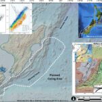
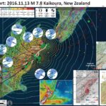
This is the first of several posts about a complex earthquake series that happened along the northern end of the South Island in New Zealand. I was at sea on the R/V Tangaroa collecting piston cores offshore along the Hikurangi subduction zone this month. While I was at sea, there was a large earthquake, probably along one of the upper plate faults in this region. I present a simple interpretive poster below and will follow up with several more posts as I find more time between my other responsibilities (I have been gone at sea for two weeks, so I have lots of catch up work to do). This earthquake series is in a complicated part of the Earth where a subduction plate boundary turns into a transform plate boundary. There was a tsunami warning for the nearby coasts, but not for a global tsunami.
Geonet is a website in New Zealand that is a collaboration between the Earthquake Commission and GNS Science. Here is the website at Geonet where one can find the most up to date observations and interpretations about this M 7.8 Kaikoura Earthquake series.

  • Below is a map that I prepared that shows the earthquakes (magnitude M ≥ 2.5) for the month of November as green circles (diameter represents earthquake magnitude). I also plot earthquakes with magnitudes M ≥ 5.5 from the period of 1950-2016. These are from the USGS NEIC, so the regional network run in New Zealand may have a larger number of earthquakes. I present two maps, one with a 250 m resolution bathymetric grid as a base and one with a Google Earth satellite based map as a base. This is not an official GNS nor NIWZ figure, but they were major supporters of the TAN163 cruise that I participated on, so we can attribute the core data to these organizations.
  • I placed the moment tensors for the larger earthquakes during this time period since the M 7.8 earthquake. The main earthquake is a compressional earthquake, probably on an upper plate fault. The M 7.8 earthquake triggered slip on other thrusts and some strike-slip faults in the region. Surface deformation measured using Interferometric Synthetic Aperture Radar (INSAR) is localized, supporting the upper plate rupture interpretation. Slip on the thrust during the 7.8 is estimated to be about 10 meters, which is also the maximum slip on some of the strike-slip fault systems. There have been some excellent photographs of the fault rupture (I will include these in a later post). Most of the large earthquakes are strike-slip, but there are some connecting faults that show thrust mechanisms. I also show the regions of different faults that have been observed to have surface ruptures.
  • After the earthquake, we changed our plans to conduct some post-earthquake response analyses. We collected additional cores to search for sedimentary evidence of the M 7.8 earthquake. We also collected sub-bottom profile and bathymetric data to search for seafloor exposed fault rupture. The cores we collected for our general study are shown as red cross-dots. The cores we collected as the earthquake are plotted as yellow cross-dots.
  • I also include the shaking intensity contours on the map. These use the Modified Mercalli Intensity Scale (MMI; see the legend on the map). This is based upon a computer model estimate of ground motions, different from the “Did You Feel It?” estimate of ground motions that is actually based on real observations. The MMI is a qualitative measure of shaking intensity. More on the MMI scale can be found here and here. This is based upon a computer model estimate of ground motions, different from the “Did You Feel It?” estimate of ground motions that is actually based on real observations.
  • I placed a moment tensor / focal mechanism legend on the poster. There is more material from the USGS web sites about moment tensors and focal mechanisms (the beach ball symbols). Both moment tensors and focal mechanisms are solutions to seismologic data that reveal two possible interpretations for fault orientation and sense of motion. One must use other information, like the regional tectonics, to interpret which of the two possibilities is more likely.
    • Inset Figures

      I include some inset figures. Here is some information about them. Below I include the original figures with the figure captions as blockquotes.

    • In the upper right corner is a map from NIWA (Phil Barnes). This map shows some of the major faults in this region. I placed the observed fault offsets on this map as orange lines. This map is on the NIWA website, but I will find the Barnes publication this came from and post that in a follow up web page.
    • In the lower right corner is a map from Geological and Nuclear Sciences (GNS) in Māori: Te Pū Ao. This map shows the regional faults and where there have been observations of surface rupture. The coseismic (during the earthquake) Global Positioning System (GPS) observations. Earthquakes are also plotted.
    • To the left of that is a figure from the Geospatial Information Authority of Japan (GSI). This is a summary figure showing modeled uplift as compared to InSAR analysis results. Note how localized the deformation is. I will present and discuss the analyses that went into this figure in a follow-up report.
    • To the left of that is a generalized tectonic map of the region.


    Here are the USGS websites for the large earthquakes plotted in the map above.

  • 20161113 M 7.8 11:02 USGS
  • 20161113 M 6.5 11:32 USGS
  • 20161113 M 6.1 11:52 USGS
  • 20161113 M 6.2 13:31 USGS
  • 20161113 M 5.7 19:28 USGS
  • 20161114 M 6.5 00:34 USGS
  • 20161114 M 5.4 01:30 USGS
  • 20161114 M 5.8 06:47 USGS
  • 20161115 M 5.4 01:34 USGS
  • 20161115 M 5.4 06:30 USGS
  • 20161118 M 5.1 14:22 USGS
  • 20161122 M 5.9 00:19 USGS
  • 20161122 M 5.3 00:19 USGS
  • 20161122 M 5.0 19:38 USGS
  • Here is an image of the seismograph as recorded by the Humboldt State University, Department of Geology, Baby Benioff seismometer. Here is a high resolution version as scanned by Dr. Stephen Tilinghast. (108 MB)

  • Here is the USGS Seismicity of the Earth map for this region (Benz et al., 2010). Click on the map for the pdf of this report (66 MB pdf). Here is 10 MB jpg file.

  • Initial recon overflights report that there have been over 100,000 landslides from this earthquake. Below is a map that shows a different analysis that people are conducting. There will be more.

  • Here is one of the early InSAR results from COMET. I will present more of these is a follow-up report.

  • Here is a cool comparison animated gif showing before and after the earthquake. This is an animated gif showing photos taken by Casey Miln and Andrew Spencer.

  • Casey Miln

  • Andrew Spencer

Earthquake Report: El Salvador!

While waiting to board my plane from Sydney (AU) to SFO, I put together an interpretive poster for the M 7.0 earthquake offshore of El Salvador from today. I will spend more time later adding more information, including some background material about this subduction zone and some of the materials that I include in this poster. Generally, I use the same type of data that I include in my other earthquake posters. I will add that information here later (need to board my plane now). Here is the USGS website for this earthquake.
I have some maps that show the historic earthquakes in this region that I will upload later (probably as an update to this initial report).
Here is my interpretive poster for the extensional earthquake that is in the downgoing (subducting) Cocos plate. This earthquake has a shallow depth and produced a small tsunami run-up.
I also include the shaking intensity contours on the map. These use the Modified Mercalli Intensity Scale (MMI; see the legend on the map). This is based upon a computer model estimate of ground motions, different from the “Did You Feel It?” estimate of ground motions that is actually based on real observations. The MMI is a qualitative measure of shaking intensity. More on the MMI scale can be found here and here. This is based upon a computer model estimate of ground motions, different from the “Did You Feel It?” estimate of ground motions that is actually based on real observations.
I placed a moment tensor / focal mechanism legend on the poster. There is more material from the USGS web sites about moment tensors and focal mechanisms (the beach ball symbols). Both moment tensors and focal mechanisms are solutions to seismologic data that reveal two possible interpretations for fault orientation and sense of motion. One must use other information, like the regional tectonics, to interpret which of the two possibilities is more likely.

    Inset Figures

    I include some inset figures. Here is some information about them. Below I include the original figures with the figure captions as blockquotes.

  • In the upper right corner is a map from Funk et al. (2009) that shows focal mechanisms for earthquakes in this region. These data are from the Harvard Centroid Moment Tensor (CMT) catalog for all earthquakes from 1976 to 2007. The region outlined in dashed red lines shows the limit for the Funk et al. (2009) summary figure in the lower right corner and the map and cross section on the left side of the poster.
  • In the lower right corner is a tectonic summary figure from Funk et al. (2009). The authors suggest that there is a forearc sliver in this region. A forearc sliver is a large plate boundary scale strike-slip fault bounded block that is formed due to strain partitioning. When the relative plate motion at a subduction zone are not perpendicular to the megathrust fault, the motion that is perpendicular is accommodated by the megathrust fault. The plate motion that is not perpendicular to the subduction zone fault is accommodated by strike-slip faults parallel to the strike of the subduction zone fault. The authors place red arrows showing the relative motion along the plate bounding fault along the eastern boundary of this forearc sliver (these are called forearc sliver faults for obvious reasons). A classic example of a forearc sliver fault is the Sumatra fault along the Sunda subduction zone. Forearc sliver faults do not always bound a block like this and are not always parallel to the plate boundary. The Cascadia subduction zone has a series of forearc sliver faults offshore, but these are formed oblique to the plate boundary. For the case in cascadia, the plate margin parallel strain is accommodated by rotating blocks, not rigid blocks. As these blocks rotate in response to this shear couple, they rotate and form strike-slip faults between the blocks (forming “bookshelf” faults). Another plate where relative oblique motion creates rotating blocks is along the Aleutian subduction zone.
  • On the left part of the poster I include a map and some cross sections (Funk et al., 2009). The map shows epicenters from 1995-2003. The locations of the cross sections B, C, D, and E are designated by red lines. Arc volcanoes plotted in the cross sections are also shown on the map. The cross sections show the hypocenters from the earthquakes plotted on the map.
  • To the right of these Funk et al. (2009) figures, I include a subset of figures from Benz et al. (2010). There is a map that shows USGS epicenters with dots colored by depth and magnitude represented by circle diameter. There is also a cross section for this region, just to the northwest of El Salvador. Cross section B-B’ shows the earthquake hypocenters along a profile displayed on the map. Note how the subduction zone dip steepens to the northeast.


  • Here is the focal mechanism summary map from Funk et al. (2009). The authors depict the forearc sliver as a shaded red region. Note the strike-slip focal mechanisms in the region on the northeast of the forearc sliver.

  • Tectonic setting of Central America displayed on satellite topography and bathymetry from Sandwell and Smith (1997). Subduction of the Cocos plate beneath the Caribbean plate occurs along the Middle America Trench. Global positioning system (GPS)–based plate velocities are relative to a fixed Caribbean plate, and focal mechanisms are from the Harvard Centroid Moment Tensor (CMT) catalog for all events from 1976 to 2007. Northwestward arc-parallel translation of the Central America forearc sliver (red shading) occurs at 7–8 mm yr–1 on Nicoya Peninsula of Costa Rica (Norabuena et al., 2004) and 14 mm yr–1 in Nicaragua (DeMets, 2001). The boundary between the Caribbean and North American plate occurs along the left-lateral strike-slip Swan Islands fault zone (SIFZ), Polochic fault (PF), and Motagua fault (MF).

  • Here is the seismicity map and cross sections for the region to the southeast of El Salvador. The subduction zone in the El Salvador region is depicted by cross section B. Note that the subduction zone has a low angle dip in the shallow region of the fault, then steepens to 55 degrees to the east.


  • (A) Earthquake locations are from the National Earthquake Information Center (NEIC) and, in Nicaragua, were recorded by the local Nicaragua network from 1995 to 2003 operated by the Instituto Nicaraguense de Estudios Territoriales (INETER ). (B–E) Earthquake profiles are perpendicular to the Middle America Trench (MAT) and extend to the interior volcanic highlands of Central America. These profiles merge all earthquakes within a 50-km-wide swath along each transect. Seismic activity beneath the volcanic front in Nicaragua is more evident because of more data from local stations of the Nicaraguan seismic network. These shallow crustal earthquakes commonly occur within the upper 30 km of the crust and are concentrated within ~25 km of the active Central America volcanic front (CAVF).

  • Here is the summary figure from Funk et al. (2009). This map shows the detailed fault mapping the authors prepared for their manuscript. Their observations include field mapping and seismic profiles. There are several parts of this forearc sliver fault system that show how the strike-slip system bends and steps. There are restraining bends (where the s-s fault generates compression) and releasing bends (where the s-s fault generates extension). These regions are colored red and green, respectively. In the Marabios En Exchelon segment of this map there are some plate margin obvlique extensional fault bounded basins. These appear to be formed by bookshelf style faulting.

  • Regional tectonic map of Central America emphasizing key structures described in this paper. The El Salvador fault zone (ESFZ) is characterized by a broad right-lateral shear zone accommodating transtensional motion that results in multiple pull-apart basins . A major transition zone occurs in the Gulf of Fonseca, where strike-slip fault zones along the Central American forearc sliver change strike from dominantly east-west strikes in El Salvador to northwesterly strikes in Nicaragua. A proposed restraining bend connects faults mapped in the Gulf of Fonseca with fault scarps deforming Cosiguina volcano and faults of the Central America volcanic front north of Lake Managua . Diffuse and poorly exposed faults parallel to the Central America volcanic front in northern Nicaraguan segment are inferred to represent a young fault boundary in which right-lateral shear is accommodated over a broad zone. This model proposes a young en echelon pattern of strike-slip and secondary faults based on secondary extensional features and fi ssure eruptions along the Marabios segment of the Central America volcanic front. Lake Managua and the Managua graben are interpreted to occur at a major releasing bend in the trend of the Nicaraguan depression and are marked by the curving surface trace of the Mateare fault interpreted from aeromagnetic data. Subsequent right-lateral strike-slip motion related to translation of the Central America forearc sliver may occur along these reactivated normal faults. The Lake Nicaragua segment of the Central America volcanic front is bounded by a normal fault (LNFZ—Lake Nicaragua fault zone) offsetting the Rivas anticline, the southeastward continuation of this normal fault into Costa Rica (CNFZ—Costa Rica fault zone), and a synthetic normal fault (SRFZ—San Ramon fault zone) that we discovered in our survey of Lake Nicaragua. Transverse faults (MFZ—Morrito fault zone, JMFZ—Jesus Maria fault zone) strike approximately east-west across the Central America volcanic front. North-south–trending rift zones are abundant in El Salvador but less common in Nicaragua and may also be controlled by regional east-west extension affecting the northwestern corner of the Caribbean plate.

  • Here is a map and cross section of seismicity that was written about an earthquake pair that happened in 2001 from Martínez-Díaz et al. (2004). In January 2001 there was a M 7.7 earthquake in the downgoing Cocos plate. In February there was a M 6.6 earthquake in the Caribbean plate, which was probably triggered by the January quake. The triggered M 6.6 quake was a strike-slip earthquake on along the plate boundary forearc sliver, the El Salvador fault zone (ESFZ). I include other figures below.
    • Here are the USGS websites for the major earthquakes discussed by Martínez-Díaz et al. (2004).
    • 1982.06.19 M 6.2 El Salvador (may have triggered an earthquake in 1986)
    • 2001.01.13 M 7.7 El Salvador
    • 1982.06.19 M 6.6 El Salvador (may have been triggered by M 7.7)


    A: Geodynamic setting of study area. Line within box indicates trace of cross sections B and C. Plate motion direction and rates are shown by arrows (data from DeMets, 2001). B: Cross section passing through coordinates 13.938N, 88.788W. Focal mechanisms were taken from Harvard Centroid Moment Tensor (CMT) and U.S. Geological Survey–National Earthquake Information Center (USGS-NEIC) catalogues (period 1977–February 2003). Gray dots are hypocenters from USGSNEIC database (Ms >2.5). Dashed lines represent estimation of upper and lower bounds of seismogenic zone of subducted slab. C: Cross section of 2001 seismic sequence of El Salvador following two main shocks of January and February. Hypocenters are from Servicio Nacional de Estudios Territoriales catalogue and focal mechanisms are from Harvard CMT and USGS-NEIC catalogues.

  • Here is a map that shows focal mechanisms for large earthquakes in the region from 1977-2001. The ESFZ is visible on the shaded relief map (the fault creates enough topography to be shown at the scale of kms).

  • Radar–Shuttle Radar Topography Mission image of El Salvador (courtesy of Jet Propulsion Laboratory) with historical destructive earthquakes (white circles) and instrumental epicenters (Ms >2.5, period 1977–2001) from U.S. Geological Survey–National Earthquake Information Center (USGS-NEIC) catalogue (small dots). Small focal mechanisms are from events with Mw >5.5 (period 1977–2001, Harvard Centroid Moment Tensor database). Large mechanisms are from Buforn et al. (2001). Inset: map of faults extracted from Geological Map of El Salvador (Bosse et al., 1978). ESFZ—El Salvador fault zone.

  • Here is a map that shows how the afershocks (of the M 6.6) were limited to two segments of the ESFZ.

  • A: Aftershocks sequence of February 2001 (Mw 6.6) event projected on Radar image of El Salvador fault zone (ESFZ). SM—San Miguel; SV—San Miguel volcano; IL—Lago Ilopango; RS—rupture segment; JC—Jucuapa; RL—Rio Lempa; RG—Rio Grande. B: Oblique view of digital elevation model of volcanic arc with ESFZ trace.

  • Here are some figures that show the modeled changes in static coulomb stress generated by earthquakes in 1982 and 2001. Regions that get increased in stress following an earthquake are plotted in red and regions that have lowered levels of stress are in blue. We do not know what the state of stress is on any fault at any given time. The changes in stress in these regions are very small compared to the stresses that faults release during earthquakes (so, the possibility that a fault my be triggered by these small changes is also very small). Generally, a fault would need to be at a high state of stress to be triggered by an earthquake in this manner.
  • Panels A, B, and C are maps showing coulomb stress changes for the 1982 series and the 2001 series. Panel D is a cross section for the 2001 sequence. Note how the 1986 and Feb 2001 faults are in regions of increased stress. Also note how the ESFZ in regions adjacent to the Feb 2001 earthquake have increased stress.

  • A–C: Models of change in static Coulomb failure stress (CFS) generated after events of 1982, January 2001, and February 2001 projected on map of faults. Black line represents El Salvador fault zone (ESFZ). D: Model for 2001 event is shown in cross section. E: Joint model with CFS change generated by three major events. Rectangles represent surface ruptures. Dotted rectangles represent hypothetical ruptures.

  • Finally, here are the hypocenters shown with a low angle oblique view. The upper figure shows aftershocks for the Jan 2001 earthquake and the lower figure shows the aftershocks for the Feb earthquake.

  • Fault planes of main shocks fitted to aftershocks of the first three days, with the epicentres and outline of El Salvador. A. Representation for the 13 January Mw 7.7 event. The fault trace is subparallel to the coast. B. Representation for the 13 February Mw 6.6 event.

  • Here is a map that shows earthquakes from the NEIC for the region from 1900 to 2016, for magnitudes greater than or equal to M 6.0. The color of the dot represents the hypocentral depth of the earhquake. Note how the earthquakes fenerally get deeper along with the subduction zone megathrust. Some do not for earthquakes in the Caribbean plate and along the Swan Islands fault zone. The lower map shows earthquakes M ≥ 7.0.
  • Here are the USGS queries I used for the maps below.
    • Earthquakes from 1900-2016 for magnitudes M ≥ 6.0 USGS
    • Earthquakes from 1900-2016 for magnitudes M ≥ 7.0 USGS


  • Here is the “seismicity of the Earth” USGS series poster for this region. Click on the thumbnail below for the pdf version (13 MB pdf).

  • Here are the tsunami model results from the Pacific Tsunami Warning Center. Note how the observations in the text report below are generally consistent with this forecast.

  • Here is the National Tsunami Warning Center (NTWC) tsunami travel-time map.

  • Here are the tsunami observations.

    References:

  • Benz, H.M., Tarr, A.C., Hayes, G.P., Villaseñor, Antonio, Furlong, K.P., Dart, R.L., and Rhea, Susan, 2011, Seismicity of the Earth 1900–2010 Caribbean plate and vicinity: U.S. Geological Survey Open-File Report 2010–1083-A, scale 1:8,000,000.
  • Funk, J., Mann, P., McIntosh, K., and Stephens, J., 2009. Cenozoic tectonics of the Nicaraguan depression, Nicaragua, and Median Trough, El Salvador, based on seismic-reflection profiling and remote-sensing data in GSA Bulletin, v. 121, no. 11/12, p. 1491-1521.
  • Martínez-Díaz, J.A., Álvarez-Gómez, J.A., Benito, B., and Hernández, D., 2004. Triggering of destructive earthquakes in El Salvador in GSA Bulletin, v. 32., no. 1, p. 65-68.

Getting ready for the cruise!

2016.11.09

Getting ready for the cruise!

My main research cruise blog page is here: http://humboldt-jay.blogspot.com.

  • We will be heading to sea to search for submarine landslide deposits called turbidites. There are several ways that these landslides can be triggered. Earthquakes are the most common landslide trigger on land and probably also in the submarine environment.
  • I have worked on turbidite Paleoseismology cruises offshore of Sumatra, Cascadia, and the Lesser Antilles. These are all places where there is an active subduction zone. I have documented these cruises on my research cruise blog humboldt-jay.blogspot.com. The research offshore of Sumatra was for my Ph.D. dissertation and is ongoing. The coring we conducted offshore of Cascadia was in support of Dr. Chris Goldfinger’s research on the spatiotemporal variation in earthquakes along the Cascadia subduction zone. Recently, we received the Kirk Bryan Award from the Geological Society of America for the USGS Professional Paper 1661-F. This past summer I participated on a French cruise aboard the NO Pourquoi Pas? The principal investigator for this Caribbean cruise was Nathalie Feuillet, from Institut de Physique du Globe de Paris (IPGP) in Paris.
  • We will be collecting sediment cores aboard the R/V Tangora, a National Institute of Water and Atmospheric Research Ltd (NIWA) research ship. R/V stands for “research vessel.” Here is the website that has information about the R/V Tangora. : www.niwa.co.nz/services/vessels/niwa-vessels/rv-tangaroa

Background

  • Below is a map that shows the general region where we plan on taking cores. The principal investigator for this cruise is Dr. Phillip Barnes, from NIWA. Dr. Barnes has done an incredible job planning for this cruise and I outline the general strategy below. As always, we will modify our plan as our experiences during the cruise inform us.
  • We will be collecting cores in sedimentary basins along the slope and in channel and other depositional settings along turbidite channel systems in the trench. We will be using classic methods (well, this is a new science, so it is funny to call these classic methods) used by many who look for seismoturbidites. We will be looking for sites that have sources of sediment that are isolated from each other. We are especially interested if these sites extend for distances larger than the length of faults that might be additional sources of ground motions that might trigger submarine landslides. We will also be looking for sites that permit us to apply the confluence test, which also requires sites that have isolated source distances that are sufficiently large.
    • I include some inset maps that have some other background material.

    • In the upper right corner is a map that shows the general plate tectonics of this region. This comes from Mike Norton via Creative Commons. The Pacific plate: Australia plate relative plate motions are shown in orange. Note how the plate motion is increasingly oblique as slip is transferred from the Kermadec-Hikurangi subduction zone systems in the north to the Alpine fault system (via Marlborough) in the south, then again to the subduction zone even further south.
    • In the upper left corner shows seismicity as plotted by Wallace, et al. (2009). These are earthquakes from 1990 through December 2007. The figure on the right shows the deeper events with their depth represented by color.
    • In the lower right corner is another figure from Wallace et al. (2009). This one shows more detailed fault mapping in the accretionary prism. These are offshore thrust faults that are additional sources of ground shaking for triggering turbidites. It will be important to be able to extend our correlations beyond any individual fault system to be able to link any given correlated turbidite to ground motions from the megathrust. There are also some strike-slip faults that may also confound our analysis, particularly in the southern Hikurangi margin. In this inset is a cross section showing that the accretionary prism is composed on imbricate thrust faults. These are the additional sources of ground shaking that are mapped in plan view on the map (labeled “Forearc domain” in the cross section).


    Here are some of the inset maps on their own, with their original figure captions as blockquotes.

  • Here is the plot from Wallace et al. (2009) that shows the seismicity from 1990-2007.

  • Selected seismicity between January 1990 and December 2007 (inclusive), from the GeoNet database (http://geonet.org.nz). Events shown are only those which were recorded by six or more stations, with nine or more observed phases, with unrestricted location depths, and RMS of arrival time residuals less than 1.0 s. Magnitude range of events shown is 0.29–6.99. (left) Events shallower than 33 km. (right) Events greater than 33-km depth.

  • Here is the map from Wallace et al. (2009) that shows the regional and local tectonics in the Hikurangi Trough.


    Tectonic setting of the Hikurangi margin. Modified from Barnes et al. [2009], copyright 2009, Elsevier. (a) Detailed bathymetry (NIWA), topography, and active faulting (black lines) of the onshore and offshore subduction margin. Dashed contours indicate sediment thickness on lower plate from Lewis et al. [1998]. Bold white dashed line shows the back of the accretionary wedge and the front of a deforming buttress of Cretaceous and Paleogene rocks covered by Miocene to Recent slope basins [from Lewis et al., 1997; Barnes et al., 1998b, 2009]. A–A0 line denotes cross-section location in Figure 1d. Dashed black lines show locations of seismic reflection lines from Figure 4, labeled by line number. White arrow shows Pacific/Australia relative plate motion in the region from Beavan et al. [2002]. Onshore active faults from GNS Science active faults database (http://maps.gns.cri.nz/website/af/). TVZ, Taupo Volcanic Zone; NIDFB, North Island Dextral Fault Belt; LR, approximate location of Lachlan Ridge; KR, approximate location of Kidnappers Ridge. (b) Broader-scale New Zealand tectonic setting. (c) Regional tectonic framework. RI, Raoul Island; NZ, New Zealand; HT, Hikurangi Trough. (d) Interpretive cross section across the strike of the subduction margin. Cross-section location denoted by A–A0 line in Figure 1a.

    Here are some figures that show the historic and prehistoric history of earthquakes in this region, with their original figure captions as blockquotes.

  • Here is a figure that shows our existing knowledge of the historic subduction zone earthquakes for this region (Wallace et al. (2014).


    Tectonic setting of the Hikurangi subduction zone at the boundary between the Pacific and Australian Plates. Black contours show the depth to the subduction interface (Williams et al., 2014). Red dots = historical subduction thrust events (all MW < 7.2). Gray dots = continuous GPS sites (http://www.geonet.org.nz). Arrows show convergence rates at the trench in mm yr–1 (Wallace et al., 2012a). PB = 1947 Poverty Bay earthquake. TB = 1947 Tolaga Bay earthquake. WF = Wairarapa Fault, the site of the 1855 earthquake. BL = Big Lagoon. MP = Mahia Peninsula. Black lines onshore are active faults (http://www.data.gns.cri.nz/af). In the forearc, most of these faults are either right lateral strike-slip or reverse. The strike-slip faults help to accommodate the margin-parallel component of relative plate motion.

  • Here is a figure that shows our existing knowledge of the prehistoric subduction zone earthquakes (Paleoseismology) for this region (Wallace et al. (2014).


    Map in upper panel shows locations of published Holocene records of coseismic vertical deformation along the Hikurangi Margin. Timeline in lower panel shows the approximate ages and types of impact found at different sites along the margin (note that this is an overview that does not show individual dates and their errors). We use black horizontal lines on the timeline to indicate times when vertical deformation occurs at multiple sites along the margin (summarized in the right panel of the timeline). These lines are also used on the map to indicate the approximate lateral extent of deformation and the strength of evidence for occurrence of a great subduction thrust earthquake. *Site 1: Clark et al. (2011) and Hayward et al. (2010). Site 2: McSaveney et al. (2006). Site 3: Berryman et al. (2011). Site 4: Hayward et al. (2006). Sites 5 and 6: Cochran et al. (2006). Site 7: Berryman (1993). Site 8: Wilson et al. (2006).

    References

  • Wallace et al., 2009. Characterizing the seismogenic zone of a major plate boundary subduction thrust: Hikurangi Margin, New Zealand, Geochem. Geophys. Geosyst., 10, Q10006, doi:10.1029/2009GC002610
  • Wallace, L.M., U.A. Cochran, W.L. Power, and K.J. Clark. 2014. Earthquake and tsunami potential of the Hikurangi subduction thrust, New Zealand: Insights from paleoseismology, GPS, and tsunami modeling. Oceanography 27(2):104–117, http://dx.doi.org/10.5670/oceanog.2014.46.

Earthquake Report: Laytonville (northern CA)!

This morning there was another earthquake in northern CA between the San Andreas (SAF) and Maacama faults (MF). This region has been active for the past few years, with earthquakes in the M 3-4 range. Most recently, there was a M 3.8 really close to today’s M 4.1. These earthquakes may indicate the possibility of an unmapped fault. There have been earthquakes in 2000, 2014, and 2015 that align along strike (of a possible fault that is sub-parallel to the SAF/MF systems). Here is the USGS website for today’s M 4.1 earthquake.
The San Andreas fault is a right-lateral strike-slip transform plate boundary between the Pacific and North America plates. The plate boundary is composed of faults that are parallel to sub-parallel to the SAF and extend from the west coast of CA to the Wasatch fault (WF) system in central Utah (the WF runs through Salt Lake City and is expressed by the mountain range on the east side of the basin that Salt Lake City is built within).
The three main faults in the region north of San Francisco are the SAF, the MF, and the Bartlett Springs fault (BSF). I also place a graphical depiction of the USGS moment tensor for this earthquake. The SAF, MF, and BSF are all right lateral strike-slip fault systems. There are no active faults mapped in the region of Sunday’s epicenter, but I interpret this earthquake to have right-lateral slip. Without more seismicity or mapped faults to suggest otherwise, this is a reasonable interpretation.
Below I plot the seismicity from the past month, with color representing depth and diameter representing magnitude (see legend). I use the USGS Quaternary fault and fold database for the faults. I outlined the Vizcaino Block, which many interpret to be a prehistoric subduction zone accretionary prism from a time before the San Andreas existed.
I also include the shaking intensity contours on the map. These use the Modified Mercalli Intensity Scale (MMI; see the legend on the map). This is based upon a computer model estimate of ground motions, different from the “Did You Feel It?” estimate of ground motions that is actually based on real observations. The MMI is a qualitative measure of shaking intensity. More on the MMI scale can be found here and here. This is based upon a computer model estimate of ground motions, different from the “Did You Feel It?” estimate of ground motions that is actually based on real observations.
I placed a moment tensor / focal mechanism legend on the poster. There is more material from the USGS web sites about moment tensors and focal mechanisms (the beach ball symbols). Both moment tensors and focal mechanisms are solutions to seismologic data that reveal two possible interpretations for fault orientation and sense of motion. One must use other information, like the regional tectonics, to interpret which of the two possibilities is more likely. Based on the moment tensor and my knowledge of the tectonics of this region, I interpret this earthquake to have had a right lateral strike slip motion along an east-west fault.

    I include some inset figures in the poster.

  • In the upper right corner I include a map from McLaughlin et al. (2012) that shows the regional faulting.
  • In the lower right corner I include generalized fault map of northern California from Wallace (1990).
  • In the lower left corner I include a map that shows the seismicity for this region since 1960, including earthquakes with magnitudes greater than or equal to M 1.5. I have labeled some of the significant earthquake swarms, with magnitudes ranging from M 3-4. Here is the USGS search that I used to create this map.
  • To the right of the seismicity map is a figure that shows the evolution of the San Andreas fault system since 30 million years ago (Ma). This is a figure from the USGS here.
  • In the upper left corner I include the Earthquake Shaking Potential map from the state of California. This is a probabilistic seismic hazard map, basically a map that shows the likelihood that there will be shaking of a given amount over a period of time. More can be found from the California Geological Survey here. I place a yellow star in the approximate location of today’s earthquake.


  • Earlier this month (a couple days ago), there was an earthquake in this region. Below is my interpretive poster for that earthquake. Here is my Earthquake Report.

  • Earlier this year, there was an earthquake in this region, along the BSF. Below is my interpretive poster for that earthquake. Here is my Earthquake Report.

  • Last year there was an earthquake in this region. Below is my interpretive poster for that earthquake. Here is my Earthquake Report.

  • I place a map shows the configuration of faults in central (San Francisco) and northern (Point Delgada – Punta Gorda) CA (Wallace, 1990). Here is the caption for this map, that is on the lower left corner of my map. Below the citation is this map presented on its own.
  • Geologic sketch map of the northern Coast Ranges, central California, showing faults with Quaternary activity and basin deposits in northern section of the San Andreas fault system. Fault patterns are generalized, and only major faults are shown. Several Quaternary basins are fault bounded and aligned parallel to strike-slip faults, a relation most apparent along the Hayward-Rodgers Creek-Maacama fault trend.


  • About 75% of the relative plate motion is accommodated along the SAF and its synthetic sister faults in the northern CA region. The rest of the plate boundary motion is accommodated along the Eastern CA shear zone and Walker Lane, along with the Central Nevada Seismic Belt, and the Wasatch fault systems. In Northern CA, there is about 33-37 mm/yr strain accumulated on the SAF plate boundary system. About 18-25 mm/yr is on the SAF, 8-11 mm/yr on the MF, and 5-7 mm/yr on the Bartlett Springs fault system (Geist and Andrews, 2000).
  • Here is a map from McLaughlin et al. (2012) that shows the regional faulting. I include the figure caption as a blockquote below.

  • Maps showing the regional setting of the Rodgers Creek–Maacama fault system and the San Andreas fault in northern California. (A) The Maacama (MAFZ) and Rodgers Creek (RCFZ) fault zones and related faults (dark red) are compared to the San Andreas fault, former and present positions of the Mendocino Fracture Zone (MFZ; light red, offshore), and other structural features of northern California. Other faults east of the San Andreas fault that are part of the wide transform margin are collectively referred to as the East Bay fault system and include the Hayward and proto-Hayward fault zones (green) and the Calaveras (CF), Bartlett Springs, and several other faults (teal). Fold axes (dark blue) delineate features associated with compression along the northern and eastern sides of the Coast Ranges. Dashed brown line marks inferred location of the buried tip of an east-directed tectonic wedge system along the boundary between the Coast Ranges and Great Valley (Wentworth et al., 1984; Wentworth and Zoback, 1990). Dotted purple line shows the underthrust south edge of the Gorda–Juan de Fuca plate, based on gravity and aeromagnetic data (Jachens and Griscom, 1983). Late Cenozoic volcanic rocks are shown in pink; structural basins associated with strike-slip faulting and Sacramento Valley are shown in yellow. Motions of major fault blocks and plates relative to fi xed North America, from global positioning system and paleomagnetic studies (Argus and Gordon, 2001; Wells and Simpson, 2001; U.S. Geological Survey, 2010), shown with thick black arrows; circled numbers denote rate (in mm/yr). Restraining bend segment of the northern San Andreas fault is shown in orange; releasing bend segment is in light blue. Additional abbreviations: BMV—Burdell Mountain Volcanics; QSV—Quien Sabe Volcanics. (B) Simplifi ed map of color-coded faults in A, delineating the principal fault systems and zones referred to in this paper.

  • Here is the figure showing the evolution of the SAF since its inception about 29 Ma. I include the USGS figure caption below as a blockquote.

  • EVOLUTION OF THE SAN ANDREAS FAULT.
    This series of block diagrams shows how the subduction zone along the west coast of North America transformed into the San Andreas Fault from 30 million years ago to the present. Starting at 30 million years ago, the westward- moving North American Plate began to override the spreading ridge between the Farallon Plate and the Pacific Plate. This action divided the Farallon Plate into two smaller plates, the northern Juan de Fuca Plate (JdFP) and the southern Cocos Plate (CP). By 20 million years ago, two triple junctions began to migrate north and south along the western margin of the West Coast. (Triple junctions are intersections between three tectonic plates; shown as red triangles in the diagrams.) The change in plate configuration as the North American Plate began to encounter the Pacific Plate resulted in the formation of the San Andreas Fault. The northern Mendicino Triple Junction (M) migrated through the San Francisco Bay region roughly 12 to 5 million years ago and is presently located off the coast of northern California, roughly midway between San Francisco (SF) and Seattle (S). The Mendicino Triple Junction represents the intersection of the North American, Pacific, and Juan de Fuca Plates. The southern Rivera Triple Junction (R) is presently located in the Pacific Ocean between Baja California (BC) and Manzanillo, Mexico (MZ). Evidence of the migration of the Mendicino Triple Junction northward through the San Francisco Bay region is preserved as a series of volcanic centers that grow progressively younger toward the north. Volcanic rocks in the Hollister region are roughly 12 million years old whereas the volcanic rocks in the Sonoma-Clear Lake region north of San Francisco Bay range from only few million to as little as 10,000 years old. Both of these volcanic areas and older volcanic rocks in the region are offset by the modern regional fault system. (Image modified after original illustration by Irwin, 1990 and Stoffer, 2006.)

    • Here is a map that shows the shaking potential for earthquakes in CA. This comes from the state of California here.
    • Earthquake shaking hazards are calculated by projecting earthquake rates based on earthquake history and fault slip rates, the same data used for calculating earthquake probabilities. New fault parameters have been developed for these calculations and are included in the report of the Working Group on California Earthquake Probabilities. Calculations of earthquake shaking hazard for California are part of a cooperative project between USGS and CGS, and are part of the National Seismic Hazard Maps. CGS Map Sheet 48 (revised 2008) shows potential seismic shaking based on National Seismic Hazard Map calculations plus amplification of seismic shaking due to the near surface soils.


      References

    • Geist, E.L. and Andrews D.J., 2000. Slip rates on San Francisco Bay area faults from anelastic deformation of the continental lithosphere, Journal of Geophysical Research, v. 105, no. B11, p. 25,543-25,552.
    • Irwin, W.P., 1990. Quaternary deformation, in Wallace, R.E. (ed.), 1990, The San Andreas Fault system, California: U.S. Geological Survey Professional Paper 1515, online at: http://pubs.usgs.gov/pp/1990/1515/
    • McLaughlin, R.J., Sarna-Wojcicki, A.M., Wagner, D.L., Fleck, R.J., Langenheim, V.E., Jachens, R.C., Clahan, K., and Allen, J.R., 2012. Evolution of the Rodgers Creek–Maacama right-lateral fault system and associated basins east of the northward-migrating Mendocino Triple Junction, northern California in Geosphere, v. 8, no. 2., p. 342-373.
    • Stoffer, P.W., 2006, Where’s the San Andreas Fault? A guidebook to tracing the fault on public lands in the San Francisco Bay region: U.S. Geological Survey General Interest Publication 16, 123 p., online at http://pubs.usgs.gov/gip/2006/16/
    • Wallace, Robert E., ed., 1990, The San Andreas fault system, California: U.S. Geological Survey Professional Paper 1515, 283 p. [https://pubs.er.usgs.gov/publication/pp1515].

Earthquake Report: Maule, Chile!

This morning there was a moderate sized earthquake below the megathrust in Chile. Here is the USGS website for this M 6.4 earthquake. Based upon the hypocentral depth, this appears to be along the megathrust fault (an “interface” event). However, the moment tensor shows extension (so this earthquake may be in the downgoing slab). Given the depth of this earthquake (deeper than the seismogenic zone, the region of the fault that can experience earthquakes, for most subduction zones), this is probably in the downgoing Nazca plate. This is a very seismically active region of the world, with a number of Great (M ≥ 8.0) earthquakes in recent years.
Below is my interpretive poster. I have plotted the epicenters (using the USGS earthquake feed kml) for the past 30 days with magnitudes 2.5 or greater, with color representing depth. I also include the slab depth contours from Hayes et al. (2012). These are the depth contours for the fault interface of the subduction zone. Today’s hypocentral depth is 90.8 km and the Hayes et al. (2012) slab contour in this region is between 80 and 100 km. I include the USGS moment tensor for this earthquake. I also plot the rupture length regions of historic earthquakes for this subduction zone in green (Beck et al., 1998 ). I present the patches for the 2010 and 2015 subduction zone earthquakes outlined in white dashed lines. Today’s earthquake happened in the region of the subduction zone that is “down-sip” from the 2010 earthquake. The 2010 earthquake would probably have loaded the fault in this region, so this M 6.4 earthquake may be related to the 2010 earthquake. However, it has been over 5 years since the 2010 earthquake. That being said, there are still aftershocks from the 2011 Tohoku-Oki earthquake (so it seems possible).
I also include the shaking intensity contours on the map. These use the Modified Mercalli Intensity Scale (MMI; see the legend on the map). This is based upon a computer model estimate of ground motions, different from the “Did You Feel It?” estimate of ground motions that is actually based on real observations. The MMI is a qualitative measure of shaking intensity. More on the MMI scale can be found here and here. This is based upon a computer model estimate of ground motions, different from the “Did You Feel It?” estimate of ground motions that is actually based on real observations.
I placed a moment tensor / focal mechanism legend on the poster. There is more material from the USGS web sites about moment tensors and focal mechanisms (the beach ball symbols). Both moment tensors and focal mechanisms are solutions to seismologic data that reveal two possible interpretations for fault orientation and sense of motion. One must use other information, like the regional tectonics, to interpret which of the two possibilities is more likely. Based on the moment tensor and my knowledge of the tectonics of this region, I interpret this earthquake to have had a right lateral strike slip motion along an east-west fault.

    I include some inset figures in the poster.

  • In the upper left corner I place a cross section from Melnick et al. (2006). This shows the prehistoric earthquake history on the left and a cross section of the subduction zone on the right. This cross section is in the region of the 2010 subduction zone earthquake.
  • In the upper right corner I include the space-time diagram from Beck et al. (1998 ) showing the along strike length of prehistoric earthquakes in the central subduction zone. The map above shows these prehistoric rupture strike lengths as green lines (labeled with green labels). The 2015 earthquake series ruptured past the southern boundary of the 1943 earthquake and about 30% into the 1922 earthquake region. There is a small gap between the 2010 and 2015 earthquake series, which aligns with the Juan Fernandez Ridge (a fracture zone in the Nazca plate; von Huene et al., 1997; Rodrigo et al., 2014). This fracture zone appears to be a structural boundary to earthquake slip patches (subduction zone segmentation), at least for some earthquakes. Beck et al. (1998 ) show that possibly two earthquakes ruptured past this boundary (1730 A.D. and possibly 1647 A.D., though that is queried). This segment boundary appears to be rather persistent for the past ~500 years
  • In the lower right corner, I include a time-space diagram from Moernaut et al. (2010). This diagram extends further south than the Beck et al. (1998) figure.
  • In the lower left corner I include an inset map from the USGS Seismicity History poster for this region (Rhea et al., 2010). There are two seismicity cross sections here as well, with their locations plotted on the map. The USGS plot these hypocenters along these two cross sections and I include those.


  • In February of this year, there was a M 6.3 earthquake near the coast which caused considerable damage. Below is my interpretive poster for that earthquake and here is my report.

  • In September through November of 2015, there was a M 8.3 earthquake further to the north. Below is my interpretive poster for that earthquake and here is my report, where I discuss the relations between the 2010, 2015, and other historic earthquakes in this region. Here is my report from September.

  • Here is a space time diagram from Beck et al. (1998 ). The 2015 earthquake occurs in the region of the 1943 and 1880 earthquakes. I updated this figure to show the latitudinal extent of the 2010 and 2015 earthquakes.

  • Here is the space-time diagram from Moernaut et al., 2010. I include their figure caption below in blockquote.

  • Fig.: Setting and historical earthquakes in South-Central Chile. Data derived from Barrientos (2007); Campos et al. (2002); Melnick et al.(2009)

  • The September 2015 earthquake series inspired me to compile some information on the historic tsunami in this region. Here is my report on those tsunami. Below I present my figure and an animation that compares these three tsunami from 1960, 2010, and 2014.
  • These three maps use the same color scale. There is not yet a map with this scale for the 2015 tsunami, so we cannot yet make the comparison.


  • Here is an animation of these three tsunami from the US NWS Pacific Tsunami Warning Center (PTWC). This is the YouTube link.

  • Here is the cross section of the subduction zone just to the south of this Sept/Nov 2015 swarm (Melnick et al., 2006). Below I include the text from the Melnick et al. (2006) figure caption as block text.

  • (A) Seismotectonic segments, rupture zones of historical subduction earthquakes, and main tectonic features of the south-central Andean convergent margin. Earthquakes were compiled from Lomnitz (1970, 2004), Kelleher (1972), Comte et al. (1986), Cifuentes (1989), Beck et al. (1998 ), and Campos et al. (2002). Nazca plate and trench are from Bangs and Cande (1997) and Tebbens and Cande (1997). Maximum extension of glaciers is from Rabassa and Clapperton (1990). F.Z.—fracture zone. (B) Regional morphotectonic units, Quaternary faults, and location of the study area. Trench and slope have been interpreted from multibeam bathymetry and seismic-reflection profiles (Reichert et al., 2002). (C) Profile of the offshore Chile margin at ~37°S, indicated by thick stippled line on the map and based on seismic-reflection profiles SO161-24 and ENAP-017. Integrated Seismological experiment in the Southern Andes (ISSA) local network seismicity (Bohm et al., 2002) is shown by dots; focal mechanism is from Bruhn (2003). Updip limit of seismogenic coupling zone from heat-fl ow measurements (Grevemeyer et al., 2003). Basal accretion of trench sediments from sandbox models (Lohrmann, 2002; Glodny et al., 2005). Convergence parameters from Somoza (1998 ).

  • In March 2015, there was some seismicity in this September/November 2015 earthquake slip region. I put together an earthquake report about those earthquake of magnitudes M = 5.0-5.3. I speculate that the 1922 earthquake region is a seismic gap. Note that this September/November 2015 earthquake region is along the southern portion of the seismic gap that I labeled on the map below. Dutchsinse can kiss my 4$$.
  • Here is a map that shows the recent swarm of ~M = 5 earthquakes. There are moment tensors for the earthquakes listed below, some recent historic subduction zone earthquakes. I placed the general along-strike distance for older historic earthquakes in green (and labeled their years). The largest earthquake ever recorded, the Mw = 9.5 Chile earthquake, had a slip patch that extends from the south of the map to just south of the 2010 earthquake swarm. The 2010 and 2014 earthquake swarm epicenters are plotted as colored circles, while most other historic earthquake epicenters are plotted as gray circles. Note how this March 2015 swarm is at the northern end of the 1922/11/11 M 8.3 earthquake. At the bottom of this page, I put a USGS graphic about what these moment tensor plots (beach balls) tell us about the earthquakes.

  • Hundreds of people died as a result of the 1922 earthquake. The USGS has more news reports about the 1922 earthquake here. There were also reports of a tsunami over 9 meters. So we know that this segment of the fault can produce large earthquakes and tsunami. However, it has been about a century since the last Great subduction zone earthquake in this region of the fault.

References:

Earthquake Report: Laytonville, CA

Last night we had an earthquake between the Maacama faults and the San Andreas fault. This region has experienced several earthquakes recently, which makes me think that there may be an unmapped fault there (there is no hydrothermal or oil industry drilling in this area that I am aware of). Here is the USGS website for this M 3.8 earthquake.
The San Andreas fault is a right-lateral strike-slip transform plate boundary between the Pacific and North America plates. The plate boundary is composed of faults that are parallel to sub-parallel to the SAF and extend from the west coast of CA to the Wasatch fault (WF) system in central Utah (the WF runs through Salt Lake City and is expressed by the mountain range on the east side of the basin that Salt Lake City is built within). There was a recent earthquake along the San Andreas fault in the Point Arena region in July of 2015.
The three main faults in the region north of San Francisco are the SAF, the MF, and the Bartlett Springs fault (BSF). Here is a map that shows Saturday’s epicenter as a red star. I also place a graphical depiction of the USGS moment tensor for this earthquake. The SAF, MF, and BSF are all right lateral strike-slip fault systems. There are no active faults mapped in the region of Saturday’s epicenter, but I interpret this earthquake to have right-lateral slip. Without more seismicity or mapped faults to suggest otherwise, this is a reasonable interpretation.
I also include the shaking intensity contours on the map. These use the Modified Mercalli Intensity Scale (MMI; see the legend on the map). This is based upon a computer model estimate of ground motions, different from the “Did You Feel It?” estimate of ground motions that is actually based on real observations. The MMI is a qualitative measure of shaking intensity. More on the MMI scale can be found here and here. This is based upon a computer model estimate of ground motions, different from the “Did You Feel It?” estimate of ground motions that is actually based on real observations.
I placed a moment tensor / focal mechanism legend on the poster. There is more material from the USGS web sites about moment tensors and focal mechanisms (the beach ball symbols). Both moment tensors and focal mechanisms are solutions to seismologic data that reveal two possible interpretations for fault orientation and sense of motion. One must use other information, like the regional tectonics, to interpret which of the two possibilities is more likely. Based on the moment tensor and my knowledge of the tectonics of this region, I interpret this earthquake to have had a right lateral strike slip motion along an east-west fault.

    I include some inset figures in the poster.

  • In the upper right corner I include a generalized fault map of northern California from Wallace (1990).
  • In the lower right corner I include the USGS Did You Feel It felt reports map.
  • In the lower left corner I include the Earthquake Shaking Potential map from the state of California. This is a probabilistic seismic hazard map, basically a map that shows the likelihood that there will be shaking of a given amount over a period of time. More can be found from the California Geological Survey here. I place a yellow star in the approximate location of today’s earthquake.
  • To the right of the shaking potential map is a map showing the latest version of the Uniform California Earthquake Rupture Forecast (UCERF). Let it be known that this is not really a forecast, and this name was poorly chosen. People cannot forecast earthquakes. However, it is still useful. The faults are colored vs. their likelihood of rupturing. More can be found about UCERF here. Note that the San Andreas fault, and her two sister faults (Maacama and Bartlett Springs), are orange-red.


  • Last year there was an earthquake in this region. Below is my interpretive poster for that earthquake. Here is my Earthquake Report.

  • Earlier this year, there was an earthquake in this region. Below is my interpretive poster for that earthquake. Here is my Earthquake Report.

  • I place a map shows the configuration of faults in central (San Francisco) and northern (Point Delgada – Punta Gorda) CA (Wallace, 1990). Here is the caption for this map, that is on the lower left corner of my map. Below the citation is this map presented on its own.
  • Geologic sketch map of the northern Coast Ranges, central California, showing faults with Quaternary activity and basin deposits in northern section of the San Andreas fault system. Fault patterns are generalized, and only major faults are shown. Several Quaternary basins are fault bounded and aligned parallel to strike-slip faults, a relation most apparent along the Hayward-Rodgers Creek-Maacama fault trend.


  • About 75% of the relative plate motion is accommodated along the SAF and its synthetic sister faults in the northern CA region. The rest of the plate boundary motion is accommodated along the Eastern CA shear zone and Walker Lane, along with the Central Nevada Seismic Belt, and the Wasatch fault systems. In Northern CA, there is about 33-37 mm/yr strain accumulated on the SAF plate boundary system. About 18-25 mm/yr is on the SAF, 8-11 mm/yr on the MF, and 5-7 mm/yr on the Bartlett Springs fault system (Geist and Andrews, 2000).
  • Here is a map from McLaughlin et al. (2012) that shows the regional faulting. I include the figure caption as a blockquote below.

  • Maps showing the regional setting of the Rodgers Creek–Maacama fault system and the San Andreas fault in northern California. (A) The Maacama (MAFZ) and Rodgers Creek (RCFZ) fault zones and related faults (dark red) are compared to the San Andreas fault, former and present positions of the Mendocino Fracture Zone (MFZ; light red, offshore), and other structural features of northern California. Other faults east of the San Andreas fault that are part of the wide transform margin are collectively referred to as the East Bay fault system and include the Hayward and proto-Hayward fault zones (green) and the Calaveras (CF), Bartlett Springs, and several other faults (teal). Fold axes (dark blue) delineate features associated with compression along the northern and eastern sides of the Coast Ranges. Dashed brown line marks inferred location of the buried tip of an east-directed tectonic wedge system along the boundary between the Coast Ranges and Great Valley (Wentworth et al., 1984; Wentworth and Zoback, 1990). Dotted purple line shows the underthrust south edge of the Gorda–Juan de Fuca plate, based on gravity and aeromagnetic data (Jachens and Griscom, 1983). Late Cenozoic volcanic rocks are shown in pink; structural basins associated with strike-slip faulting and Sacramento Valley are shown in yellow. Motions of major fault blocks and plates relative to fi xed North America, from global positioning system and paleomagnetic studies (Argus and Gordon, 2001; Wells and Simpson, 2001; U.S. Geological Survey, 2010), shown with thick black arrows; circled numbers denote rate (in mm/yr). Restraining bend segment of the northern San Andreas fault is shown in orange; releasing bend segment is in light blue. Additional abbreviations: BMV—Burdell Mountain Volcanics; QSV—Quien Sabe Volcanics. (B) Simplifi ed map of color-coded faults in A, delineating the principal fault systems and zones referred to in this paper.

  • Here is a map that shows the shaking potential for earthquakes in CA. This comes from the state of California here.
  • Earthquake shaking hazards are calculated by projecting earthquake rates based on earthquake history and fault slip rates, the same data used for calculating earthquake probabilities. New fault parameters have been developed for these calculations and are included in the report of the Working Group on California Earthquake Probabilities. Calculations of earthquake shaking hazard for California are part of a cooperative project between USGS and CGS, and are part of the National Seismic Hazard Maps. CGS Map Sheet 48 (revised 2008) shows potential seismic shaking based on National Seismic Hazard Map calculations plus amplification of seismic shaking due to the near surface soils.


    References

  • Geist, E.L. and Andrews D.J., 2000. Slip rates on San Francisco Bay area faults from anelastic deformation of the continental lithosphere, Journal of Geophysical Research, v. 105, no. B11, p. 25,543-25,552.
  • McLaughlin, R.J., Sarna-Wojcicki, A.M., Wagner, D.L., Fleck, R.J., Langenheim, V.E., Jachens, R.C., Clahan, K., and Allen, J.R., 2012. Evolution of the Rodgers Creek–Maacama right-lateral fault system and associated basins east of the northward-migrating Mendocino Triple Junction, northern California in Geosphere, v. 8, no. 2., p. 342-373.
  • Wallace, Robert E., ed., 1990, The San Andreas fault system, California: U.S. Geological Survey Professional Paper 1515, 283 p. [http://pubs.usgs.gov/pp/1988/1434/].

Earthquake Report: Oregon

We just had an earthquake with an epicenter that plots near Warrenton, Oregon (at the northwesternmost tip of Oregon, near the mouth of the Columbia River). Here is the USGS website for this M 3.5 earthquake. Even though it is a small earthquake, it was felt by many (almost 200 people).
This earthquake has an epicentral depth of ~38 km, well below the megathrust fault at this location. So, this earthquake is in the downgoing oceanic lithosphere related to the Juan de Fuca plate.
Below is my interpretive poster map that shows the epicenter, along with the shaking intensity contours offshore and intensity data onshore. These contours use the Modified Mercalli Intensity (MMI) scale. The MMI is a qualitative measure of shaking intensity. More on the MMI scale can be found here and here. This is based upon a computer model estimate of ground motions, different from the “Did You Feel It?” estimate of ground motions that is actually based on real observations.
I also label the cities of Seattle and Portland, as well as the three visible Cascades Volcanoes.
I placed a moment tensor / focal mechanism legend on the poster. There is more material from the USGS web sites about moment tensors and focal mechanisms (the beach ball symbols). Both moment tensors and focal mechanisms are solutions to seismologic data that reveal two possible interpretations for fault orientation and sense of motion. One must use other information, like the regional tectonics, to interpret which of the two possibilities is more likely. There is no moment tensor for this earthquake, but I place a synthetic moment tensor for the CSZ in the lower part of my poster.

    I have placed several inset figures.

  • In the upper right corner is a map of the Cascadia subduction zone (CSZ) and regional tectonic plate boundary faults. This is modified from several sources (Chaytor et al., 2004; Nelson et al., 2004)
  • In the lower left corner I include a space-time diagram that shows our current knowledge of the timing of past eruptions for the Cascade Magmatic Arc (Myers and Driedger, 2008).


  • Here is the USGS “Did You Feel It?” felt report map. This map uses the MMI scale to represent the observations that people made and reported using the USGS website here.

  • This shows how these reports (represented by green dots) are evidence that the ground shaking attenuates (“lessens”) with distance from the earthquake.

  • Below is a figure from McCrory et al. (2012) that shows historic seismicity for the Cascadia subduction zone. This is the seismicity that they used to formulate the location of the megathrust fault presented in the following figures. I include their figure caption below the text in blockquote.

  • Location map showing uneven distribution of epicenters interpreted to be Wadati-Benioff earthquakes beneath the Cascadia subduction boundary colored by depth range. Earthquakes compiled from ANSS (1975–2009) and CNSN (1985–2009) catalogs based on Juan de Fuca slab model shown in Figure 4a. Transverse Mercator projection, WGS 84 standard parallel 128, centered at 46.8, 128, with standard parallel rotated 3 clockwise of vertical (plate boundaries from Wilson [2002]).

  • Below is a figure from McCrory et al. (2012) that shows the slab contours, as they interpret them, for the Cascadia subduction zone. For some reason, these slab contours were removed from the Hayes et al. (2012) USGS slab 1.0 Google Earth kml file (they used to be there, but are not longer there). There are three figures and are all part of McCrory et al. (2012) figure 4. I include their figure caption below the text in blockquote.

  • Map showing hand-contoured model of the Juan de Fuca slab surface (see text for description) and seismicity (ANSS, 1975–2009; CNSN, 1985–2009) located beneath the modeled surface. Solid lines denote depth contours in 10 km increments, long dashed lines denote supplemental depth contours in 5 km increments; short dashed lines denote interpolated contours where control points are more than 50 km apart. Note that Wadati-Benioff zone seismicity mainly occurs in regions where slab model arches along strike.


    Map showing hand-contoured model the Juan de Fuca slab surface and seismicity located in the Cascadia forearc above the slab surface.


    Map showing smoothed polynomial spline version of slab model. Solid lines denote depth contours in 10 km increments; long dashed lines denote supplemental depth contours in 5 km increments; short dashed lines denote extrapolated contours.


    References:

  • Atwater, B.F., Musumi-Rokkaku, S., Satake, K., Tsuju, Y., Eueda, K., and Yamaguchi, D.K., 2005. The Orphan Tsunami of 1700—Japanese Clues to a Parent Earthquake in North America, USGS Professional Paper 1707, USGS, Reston, VA, 144 pp.
  • Chaytor, J.D., Goldfinger, C., Dziak, R.P., and Fox, C.G., 2004. Active deformation of the Gorda plate: Constraining deformation models with new geophysical data: Geology v. 32, p. 353-356.
  • Dengler, L.A., Moley, K.M., McPherson, R.C., Pasyanos, M., Dewey, J.W., and Murray, M., 1995. The September 1, 1994 Mendocino Fault Earthquake, California Geology, Marc/April 1995, p. 43-53.
  • McCrory, P.A., Blair, J.L., Waldhauser, F., and Oppenheimer, D.H., 2012, Juan de Fuca slab geometry and its relation to Wadati-Benioff zone seismicity: Journal of Geophysical Research, v. 117, n. B09306, 23 pp., doi:10.1029/2012JB009407.
  • Myers, Bobbie, and Driedger, Carolyn, 2008, Eruptions in the Cascade Range during the past 4,000 years: U.S. Geological Survey General Information Product 63, 1 sheet [http://pubs.usgs.gov/gip/63/].
  • Nelson, A.R., Asquith, A.C., and Grant, W.C., 2004. Great Earthquakes and Tsunamis of the Past 2000 Years at the Salmon River Estuary, Central Oregon Coast, USA: Bulletin of the Seismological Society of America, Vol. 94, No. 4, pp. 1276–1292
  • Rollins, J.C. and Stein, R.S., 2010. Coulomb stress interactions among M ≥ 5.9 earthquakes in the Gorda deformation zone and on the Mendocino Fault Zone, Cascadia subduction zone, and northern San Andreas Fault: Journal of Geophysical Research, v. 115, B12306, doi:10.1029/2009JB007117, 2010.