Earthquake Report: Italy Update #1!

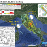
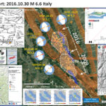
Here is an update to the #EarthquakeReport for the M 6.6 earthquake that hit Italy early this morning my time. Ironically, I was preparing a report for earthquakes in the western Pacific for my class when this M 6.6 earthquake hit and I did not notice the USGS email because I was so engaged with the western Pacific report. Here is the interpretive poster for that region over the past week or so.
This region has been experiencing a series of large earthquakes since August 2016, possibly culminating in this M 6.6 earthquake. These earthquakes may load adjacent faults in the region, so this may not be over. Given the series of earthquakes in the region further to the north (from 1916-1920), this may not be over. Stay tuned and stay safe!
The M 6.1 earthquake happened following the M 5.5 earthquake, so people had already been staying outside of their houses. This is thought to be why the casualty number was lower than expected for the M 6.1 earthquake. While the damage estimates are likely to be closer to the bar for both the M 6.1 and M 6.6 earthquakes, the casualty list is also thought to be lower for the M 6.6 earthquake for the same reason.

Below is a poster that shows epicenters from 2008 – 2016. I have included moment tensors for the largest megnitude earthquakes and outlined the region that has had earthquakes in the two periods (2009 & 2016). I also include the fault database from the Instituto Nazionale di Geofisica e Vulcanologia (the Database of Individual Seismogenic Sources, DISS v. 3.; DISS Working Group, 2015). There is a DISS legend to the right of the moment tensor legend. The Mt Vettore fault is considered a “Debated Seismogenic Source” in this database and is the blue fault line on the northern part of the 2016 rupture region.
I placed a moment tensor / focal mechanism legend on the poster. There is more material from the USGS web sites about moment tensors and focal mechanisms (the beach ball symbols). Both moment tensors and focal mechanisms are solutions to seismologic data that reveal two possible interpretations for fault orientation and sense of motion. One must use other information, like the regional tectonics, to interpret which of the two possibilities is more likely. The tectonics of this region has many normal (extensional) faults, which explain the extensional moment tensor.

    I include some inset figures and maps.

  • In the upper left corner is a map that shows seismicity for this region on maps and cross sections (Boncio et al., 2004). I placed orange stars in the approximate location of the October, 2016 earthquakes. These earthquakes happen to appear right on the center of cross section b (the lowermost cross section on the right). It appears that these earthquakes are rupturing along the Mt. Vettore fault.
  • In the upper right corner I include a map and cross section compiled by Istituto Nazionale di Geofisica e Vulcanologia (INGV). The map and cross section are from Pierantoni et al. (2013). The cross sectional focal mechanism is located in the approximate location on the cross section. Stars designate the epicentral locations for the recent seismicity on the map. This hypothesis for which structures these earthquakes are appearing on is consistent with my interpretation shown on the Boncio et al. (2004) map and cross section.
  • In the lower right corner is another map from INGV that shows the mapped faults in this region and the location of hte 2016.10.30 M 6.6 earthquake, along with other October 2016 seismicity. Observations of potential surface rupture have occurred in the region labeled “Surface faulting.”
  • In the lower left corner is another map from INGV that shows epicenters discriminated by time (August = blue, 72 hours = yeallow, 24 hours = orange, 1 hour = red). Note the overlap not seen in my main map. The local seismic network that INGV uses shows many more earthquakes than the global network contributing to the USGS database.
  • Along the base of the poster I include “USGS Did You Feel It?” maps for the 4 largest earthquakes plotted on this map.


  • Here is an animation from INGV that shows seismicity over time. This gif is from here. “This video shows the spatial distribution of simica sequence from 24 August to 31 October.”

  • Here is a European Space Agency plot that shows LOS displacement for the 30 Oct earthquake, sourced from here. “Areas in red shifted 15 inches (40 cm) toward the perspective of the satellite, while areas in blue moved away to a similar degree. (Copernicus Sentinel/ESA/CNR-IREA).

  • Here are some views of the damage from news organizations.
  • BBC
  • BBC
  • BBC
  • As a reminder, this region is in a seismically hazardous region of Italy. Here is the 10% probability of exceedance map (for 50 yrs) from INGV.

  • This is another view of the seismic hazard in Europe (Giardini et al., 2013).

  • Boncio et a. (2004) present a remarkable assessment of the seismic hazard in this region based on a 3-D model for seismogenic sources. I present some of their figures below. I include their original figure captions as blockquotes.
  • This map shows a detailed view of the normal faults in the region. Today’s earthquake is in the region shown in box 3, east of the Umbra Valley.

  • Digital elevation model of central Italy with active normal faults of the Umbria-Marche-Abruzzo Apennines and parameters of active stress tensors obtained by inversion of focal mechanisms of background microseismicity (1), aftershock sequences (2, 3, 4, 5) or striated active faults in seismic areas (6); stress data from Brozzetti and Lavecchia (1994), Boncio and Lavecchia (2000a) and Pace et al. (2002a); the stress axes are given as trend (first three numbers) and plunge (last two numbers).

  • This map shows an even more detailed and large scale view of the faults and seismicity in this region. Today’s earthquakes align to the north of Norcia, approximately along the cross section labeled “sec B.” The two cross sections are in the lower right part of the figure, with section B the lowermost cross section. Today’s earthquake may be on the AF2, the C-NFs (Colfiorito-Norcia fault systems), or MVf (Mt. Vettore fault). The AF2 fault is a proposed low angle detachment fault. These types of faults are controversial in that there are arguments about whether they are seismogenic or not. This year’s Pacific Cell Friends of the Pleistocene field trip in Panamint Valley presented research results that attempted to address this question. In Panamint Valley there are faults that have similar configurations as these faults in Italy.

  • Geological cross sections from seismic reflection profiles across the Gubbio, Gualdo T. and Colfiorito seismic areas (from Boncio et al., 1998; Boncio and Lavecchia, 2000b); epi- and hypocentral distribution of back-ground microseismicity recorded in the Umbria-Marche Apennines and rheological profiles (strength envelopes in critical stress difference, σ1–σ3) built for two different thermal contexts (50 and 40 mW/m2 surface heat flow, see Figure 3 for location); the depth of the brittle-plastic transition on rheological profiles is indicated by arrows; the used rheological parameters are indicated: crustal layering is from DSS data; A (empirical material constant), n (stress exponent) and E (activation energy) are creep parameters; ´ε = longitudinal strain rate (calculated by balancing of a regional geologic section; Figure 5 in Boncio et al., 2000); see text for further details.

  • This map shows a smaller scaled view (than the above figure) with focal mechanisms and cross sections (with structural interpretations). Hypocenters are also plotted on these cross sections. Today’s earthquakes are just south of cross section b. (earthquakes happened here in 1997)

  • Epicentres of the major seismic sequences of the last twenty years (Gubbio, 1984; Colfiorito, 1997; Norcia, 1979; Sangro, 1984) plus three small seismic sequences in the L’Aquila area (1992, 1994 and 1996); seismotectonic sections and rheological profiles built according to the local thermal context. The dashed line (sections ‘a’ and ‘b’) represents the AF low-angle extensional detachment; arrows in seismotectonic sections indicate the maximum depth-extent of the activated seismogenic faults as suggested by the best defined aftershock volume; rheological parameters as in Figure 7; in the southern Abruzzo area, creep strengths for geologic and geodetic longitudinal strain rates are compared (geologic strain rate calculated from data of Galadini and Galli, 2000; geodetic strain rate from D’Agostino et al., 2001); seismological data from Amato et al. (1998); Boncio (1998); Boncio et al. (2004); Cattaneo et al. (2000); De Luca et al. (2000); Deschamps et al. (1984); Ekstrom et al. (1998); Haessler et al. (1988); Harvard CMT database at www.seismology.harvard.edu.

Earthquake Report: Italy!

There was just another earthquake in Italy. This one is a larger magnitude M = 6.6. This region has been especially seismically active since August 2016.

This earthquake is north of the region that had an M 6.3 earthquake in 2009 that led to an interesting (putting it nicely) interaction between scientists, public employees/politicians, and the legal system. Basically, several seismologists were sentenced to prison. More on this is found online, for example, here and here.
Below is my interpretive map that shows the epicenter, along with the shaking intensity contours. These contours use the Modified Mercalli Intensity (MMI) scale. The MMI is a qualitative measure of shaking intensity. More on the MMI scale can be found here and here. This is based upon a computer model estimate of ground motions, different from the “Did You Feel It?” estimate of ground motions that is actually based on real observations. There is a legend for MMI intensities in the upper part of the interpretive poster below.
I placed a moment tensor / focal mechanism legend on the poster. There is more material from the USGS web sites about moment tensors and focal mechanisms (the beach ball symbols). Both moment tensors and focal mechanisms are solutions to seismologic data that reveal two possible interpretations for fault orientation and sense of motion. One must use other information, like the regional tectonics, to interpret which of the two possibilities is more likely. The tectonics of this region has many normal (extensional) faults, which explain the extensional moment tensor.

    I include some inset figures and maps.

  • In the upper left corner I include estimates of damage to people (possible fatalities) and their belongings from the Rapid Assessment of an Earthquake’s Impact (PAGER) report. More on the PAGER program can be found here. An explanation of a PAGER report can be found here. PAGER reports are modeled estimates of damage. On the top is a histogram showing estimated casualties and on the right is an estimate of possible economic losses. This PAGER report suggests that there will be quite a bit of damage from this earthquake (and casualties). This earthquake has a high probability of damage to people and their belongings.
  • In the upper right corner is a map showing the faulting mapped in the region surrounding and including Italy (Billi et al., 2006). There is a convergent plate boundary along the eastern part of Italy (part of the Alpide belt, a convergent boundary that extends from the Straits of Gibraltar to Australia). This fault system dips westward and is onshore in the south, but extends offshore into the Adriatic Sea in central-northern Italy. In the central part of Italy is a series of north-northwest striking extensional faults. It is these extensional (normal) faults that are responsible for the damaging seismicity in this region of central Italy. This includes the 1915, 1997, 2009, and 2016 earthquakes.
  • To the right of the Billi et al. (2006) fault map is a plot showing the seismicity from the last year. Today’s earthquakes are plotted as orange circles and the epicenters from August are plotted as gray circles.
  • To the left of this map is a figure that shows the median PGA (Peak Ground Acceleration, units of g where g = 9.8 m/s2) that has a 10% probability of exceedance (PE) in the next 50 years. This model assumes a Vs30 greater than 800 m/s. Vs is the average seismic velocity in the upper 30 meters. Vs30 is a proxy used for global to regional estimates of seismic hazard.I include their original figure captions as blockquote. This is from Stucchi et al., 2011.
  • In the lower right corner are two panels with results from the USGS “Did You Feel It?” website. The upper panel shows results from felt reports. The circles are colored vs. MMI intensity. The lower panel is a plot that shows these reports as their MMI values vary with distance from the earthquake (the horizontal axis). There are Ground Motion Prediction Equations that are empirical models (that model shaking intensity vs. distance) that are used to estimate shaking for this earthquake. The output from this model is the source of data for the shakemaps and the PAGEr damage estimates. Note how the attenuation relations (how the seismic energy is absorbed with distance from the earthquake) fit the green line (GMPE relations for lithosphere and earthquakes in California).
  • In the lower left corner is a map that shows seismicity for this region on maps and cross sections. I placed orange stars in the approximate location of the October, 2016 earthquakes. These earthquakes happen to appear right on the center of cross section b (the lowermost cross section on the right). It appears that these earthquakes are rupturing along the Mt. Vettore fault.


  • Here is the shaking intensity map (using the MMI color scale).

  • This is the GMPE regression for the above map.

  • Here is the USGS PAGER alert.

    Here are some other maps that might help. (well, one so far)

  • This Billi et al. (2006) map shows some of these west dipping normal faults in central Italy, just south of the Apennines.

  • There are some excellent maps and figures from a study from 2004 (Boncio et al, 2004). This material was posted on twitter here.
  • Below is my interpretive poster from the earthquakes from a few days ago. For more information about the figures displayed on this poster, here is the complete report for this swarm.

  • Here is a map that shows the earthquakes from the past few months, for magnitudes greater than or equal to M = 2.5. Note the M 6.6 earthquake (the largest orange circle) is between the 2016.08.23 M 6.2 earthquake (the largest gray circle in the south) and the 2016/10/28 M 6.2 earthquake (the largest yellow circle in the north).

  • Boncio et a. (2004) present a remarkable assessment of the seismic hazard in this region based on a 3-D model for seismogenic sources. I present some of their figures below. I include their original figure captions as blockquotes.
  • This map shows a detailed view of the normal faults in the region. Today’s earthquake is in the region shown in box 3, east of the Umbra Valley.

  • Digital elevation model of central Italy with active normal faults of the Umbria-Marche-Abruzzo Apennines and parameters of active stress tensors obtained by inversion of focal mechanisms of background microseismicity (1), aftershock sequences (2, 3, 4, 5) or striated active faults in seismic areas (6); stress data from Brozzetti and Lavecchia (1994), Boncio and Lavecchia (2000a) and Pace et al. (2002a); the stress axes are given as trend (first three numbers) and plunge (last two numbers).

  • This map shows an even more detailed and large scale view of the faults and seismicity in this region. Today’s earthquakes align to the north of Norcia, approximately along the cross section labeled “sec B.” The two cross sections are in the lower right part of the figure, with section B the lowermost cross section. Today’s earthquake may be on the AF2, the C-NFs (Colfiorito-Norcia fault systems), or MVf (Mt. Vettore fault). The AF2 fault is a proposed low angle detachment fault. These types of faults are controversial in that there are arguments about whether they are seismogenic or not. This year’s Pacific Cell Friends of the Pleistocene field trip in Panamint Valley presented research results that attempted to address this question. In Panamint Valley there are faults that have similar configurations as these faults in Italy.

  • Geological cross sections from seismic reflection profiles across the Gubbio, Gualdo T. and Colfiorito seismic areas (from Boncio et al., 1998; Boncio and Lavecchia, 2000b); epi- and hypocentral distribution of back-ground microseismicity recorded in the Umbria-Marche Apennines and rheological profiles (strength envelopes in critical stress difference, σ1–σ3) built for two different thermal contexts (50 and 40 mW/m2 surface heat flow, see Figure 3 for location); the depth of the brittle-plastic transition on rheological profiles is indicated by arrows; the used rheological parameters are indicated: crustal layering is from DSS data; A (empirical material constant), n (stress exponent) and E (activation energy) are creep parameters; ´ε = longitudinal strain rate (calculated by balancing of a regional geologic section; Figure 5 in Boncio et al., 2000); see text for further details.

  • This map shows a smaller scaled view (than the above figure) with focal mechanisms and cross sections (with structural interpretations). Hypocenters are also plotted on these cross sections. Today’s earthquakes are just south of cross section b. (earthquakes happened here in 1997)

  • Epicentres of the major seismic sequences of the last twenty years (Gubbio, 1984; Colfiorito, 1997; Norcia, 1979; Sangro, 1984) plus three small seismic sequences in the L’Aquila area (1992, 1994 and 1996); seismotectonic sections and rheological profiles built according to the local thermal context. The dashed line (sections ‘a’ and ‘b’) represents the AF low-angle extensional detachment; arrows in seismotectonic sections indicate the maximum depth-extent of the activated seismogenic faults as suggested by the best defined aftershock volume; rheological parameters as in Figure 7; in the southern Abruzzo area, creep strengths for geologic and geodetic longitudinal strain rates are compared (geologic strain rate calculated from data of Galadini and Galli, 2000; geodetic strain rate from D’Agostino et al., 2001); seismological data from Amato et al. (1998); Boncio (1998); Boncio et al. (2004); Cattaneo et al. (2000); De Luca et al. (2000); Deschamps et al. (1984); Ekstrom et al. (1998); Haessler et al. (1988); Harvard CMT database at www.seismology.harvard.edu.

  • Here is a poster that shows the seismic hazard for Europe (Giardini et al., 2013).

  • Here is a more detailed seismic hazard map for Italy (Stucchi et al., 2011). This shows the median PGA (Peak Ground Acceleration, units of g where g = 9.8 m/s2) that has a 10% probability of exceedance (PE) in the next 50 years. This model assumes a Vs30 greater than 800 m/s. Vs is the average seismic velocity in the upper 30 meters. Vs30 is a proxy used for global to regional estimates of seismic hazard.I include their original figure captions as blockquote.

  • The seismic hazard map showing the PGA distribution with 10% probability of exceedance in 50 years, computed on hard ground (VS30 > 800 m=s).

Earthquake Report: Mendocino fault!

Yesterday there was an earthquake along the eastern extension of the Mendocino fault system. This magnitude M = 4.1 earthquake (here is the USGS website for this earthquake) is a small magnitude, but it was widely felt. I was in Manila (CA) at the time, so I am surprised that I did not feel it. I was in the bath at the time, so maybe my shampooing was too energetic?
This earthquake appears to have occurred along the Mendocino fault, a right-lateral (dextral) transform plate boundary. This plate boundary connects the Gorda ridge and Juan de Fuca rise spreading centers with their counterparts in the Gulf of California, with the San Andreas strike-slip fault system. Transform plate boundaries are defined that they are strike-slip and that they connect spreading ridges. In this sense of the definition, the Mendocino fault and the San Andreas fault are part of the same system. This earthquake appears to have occurred in a region of the Mendocino fault that ruptured in 1994. See the figures from Rollins and Stein below.
Below is my interpretive map that shows the epicenter, along with the shaking intensity contours. These contours use the Modified Mercalli Intensity (MMI) scale. The MMI is a qualitative measure of shaking intensity. More on the MMI scale can be found here and here. This is based upon a computer model estimate of ground motions, different from the “Did You Feel It?” estimate of ground motions that is actually based on real observations.
I placed a moment tensor / focal mechanism legend on the poster. There is more material from the USGS web sites about moment tensors and focal mechanisms (the beach ball symbols). Both moment tensors and focal mechanisms are solutions to seismologic data that reveal two possible interpretations for fault orientation and sense of motion. One must use other information, like the regional tectonics, to interpret which of the two possibilities is more likely. Based on the moment tensor and my knowledge of the tectonics of this region, I interpret this earthquake to have had a right lateral strike slip motion along an east-west fault.

    I have placed several inset figures.

  • In the upper right corner is a map of the Cascadia subduction zone (CSZ) and regional tectonic plate boundary faults. This is modified from several sources (Chaytor et al., 2004; Nelson et al., 2004)
  • Below the CSZ map is an illustration modified from Plafker (1972). This figure shows how a subduction zone deforms between (interseismic) and during (coseismic) earthquakes. Today’s earthquake did not occur along the CSZ, so did not produce crustal deformation like this. However, it is useful to know this when studying the CSZ.
  • In the lower left corner is a map from Rollins and Stein (2010), showing their interpretations of different historic earthquakes in the region. This was published in response to the January 2010 Gorda plate earthquake. Today’s earthquake is near the 1983 earthquake.
  • Above the Rollins and Stein figure are two USGS plots. The upper plot shows a map displaying the “Did You Feel It?” felt reports. The color scale is the same as for the MMI legend in the upper left corner. The lower plot shows how the shaking intensity attenuates (diminishes) with distance from the epicenter.


  • Here is a map from Rollins and Stein, showing their interpretations of different historic earthquakes in the region. This was published in response to the January 2010 Gorda plate earthquake. The faults are from Chaytor et al. (2004). The 1980, 1992, 1994, 2005, and 2010 earthquakes are plotted and labeled. I did not mention the 2010 earthquake, but it most likely was just like 1980 and 2005, a left-lateral strike-slip earthquake on a northeast striking fault.

  • Here is a large scale map of the 1983 earthquake swarm. The mainshock epicenter is a black star and epicenters are denoted as white circles. Note how the aftershocks trend slightly southeast in this region. Today’s swarm does the same (and the moment tensor also shows a slightly southeast strike). Note how the interpreted fault dips slightly to the north, which is the result of north-south compression from the relative northward motion of the Pacific plate.

  • Here is a large scale map of the 1994 earthquake swarm. The mainshock epicenter is a black star and epicenters are denoted as white circles.

  • Here is a plot of focal mechanisms from the Dengler et al. (1995) paper in California Geology.

  • In this map below, I label a number of other significant earthquakes in this Mendocino triple junction region. Another historic right-lateral earthquake on the Mendocino fault system was in 1994. There was a series of earthquakes possibly along the easternmost section of the Mendocino fault system in late January 2015, here is my post about that earthquake series.

  • The Gorda and Juan de Fuca plates subduct beneath the North America plate to form the Cascadia subduction zone fault system. In 1992 there was a swarm of earthquakes with the magnitude Mw 7.2 Mainshock on 4/25. Initially this earthquake was interpreted to have been on the Cascadia subduction zone (CSZ). The moment tensor shows a compressional mechanism. However the two largest aftershocks on 4/26/1992 (Mw 6.5 and Mw 6.7), had strike-slip moment tensors. These two aftershocks align on what may be the eastern extension of the Mendocino fault.
  • There have been several series of intra-plate earthquakes in the Gorda plate. Two main shocks that I plot of this type of earthquake are the 1980 (Mw 7.2) and 2005 (Mw 7.2) earthquakes. I place orange lines approximately where the faults are that ruptured in 1980 and 2005. These are also plotted in the Rollins and Stein (2010) figure above. The Gorda plate is being deformed due to compression between the Pacific plate to the south and the Juan de Fuca plate to the north. Due to this north-south compression, the plate is deforming internally so that normal faults that formed at the spreading center (the Gorda Rise) are reactivated as left-lateral strike-slip faults. In 2014, there was another swarm of left-lateral earthquakes in the Gorda plate. I posted some material about the Gorda plate setting on this page.
  • There are three types of earthquakes, strike-slip, compressional (reverse or thrust, depending upon the dip of the fault), and extensional (normal). Here is are some animations of these three types of earthquake faults. Many of the earthquakes people are familiar with in the Mendocino triple junction region are either compressional or strike slip. The following three animations are from IRIS.
  • Strike Slip:

    Compressional:

    Extensional:

  • This figure shows what a transform plate boundary fault is. Looking down from outer space, the crust on either side of the fault moves side-by-side. When one is standing on the ground, on one side of the fault, looking across the fault as it moves… If the crust on the other side of the fault moves to the right, the fault is a “right lateral” strike slip fault. The Mendocino and San Andreas faults are right-lateral (dextral) strike-slip faults. I believe this is from Pearson Higher Ed.


    References:

  • Atwater, B.F., Musumi-Rokkaku, S., Satake, K., Tsuju, Y., Eueda, K., and Yamaguchi, D.K., 2005. The Orphan Tsunami of 1700—Japanese Clues to a Parent Earthquake in North America, USGS Professional Paper 1707, USGS, Reston, VA, 144 pp.
  • Chaytor, J.D., Goldfinger, C., Dziak, R.P., and Fox, C.G., 2004. Active deformation of the Gorda plate: Constraining deformation models with new geophysical data: Geology v. 32, p. 353-356.
  • Dengler, L.A., Moley, K.M., McPherson, R.C., Pasyanos, M., Dewey, J.W., and Murray, M., 1995. The September 1, 1994 Mendocino Fault Earthquake, California Geology, Marc/April 1995, p. 43-53.
  • Nelson, A.R., Asquith, A.C., and Grant, W.C., 2004. Great Earthquakes and Tsunamis of the Past 2000 Years at the Salmon River Estuary, Central Oregon Coast, USA: Bulletin of the Seismological Society of America, Vol. 94, No. 4, pp. 1276–1292
  • Rollins, J.C. and Stein, R.S., 2010. Coulomb stress interactions among M ≥ 5.9 earthquakes in the Gorda deformation zone and on the Mendocino Fault Zone, Cascadia subduction zone, and northern San Andreas Fault: Journal of Geophysical Research, v. 115, B12306, doi:10.1029/2009JB007117, 2010.

Earthquake Report: Tyrrhenian Sea!

There was just a very deep earthquake along a small subduction zone in the Mediterranean Sea. This subduction zone is formed along the southern coast of Italy where the Ionian plate subducts to the north. This subduction zone is part of the Alpide Belt, a convergent boundary that extends from the Straits of Gibraltar to Australia. The Alpide Belt is responsibel for some of the largest mountain peaks in the world (in the European Alps and the Himalayas). Here is the USGS website for today’s M 5.8 earthquake.

Below is my interpretive map that shows the epicenter, along with the shaking intensity contours. These contours use the Modified Mercalli Intensity (MMI) scale. The MMI is a qualitative measure of shaking intensity. More on the MMI scale can be found here and here. This is based upon a computer model estimate of ground motions, different from the “Did You Feel It?” estimate of ground motions that is actually based on real observations. There is a legend for MMI intensities in the upper part of the interpretive poster below. The contours are difficult to see, but there is a small region (above the label for the Tyrrhenian Sea) of MMI II. There was only one felt report for this earthquake, probably due to its depth.
I placed a moment tensor / focal mechanism legend on the poster. There is more material from the USGS web sites about moment tensors and focal mechanisms (the beach ball symbols). Both moment tensors and focal mechanisms are solutions to seismologic data that reveal two possible interpretations for fault orientation and sense of motion. One must use other information, like the regional tectonics, to interpret which of the two possibilities is more likely. Today’s earthquake is likely due to extension in the subducting Ionian plate.

    I include some inset figures and maps.

  • In the upper right corner I include a map that shows the USGS epicenters for earthquakes with magnitudes M ≥ 4.5 from 1900-2016. There is an animation of these earthquakes below. The epicenters are plotted with the same colors as the main map (the depth color legend is in the upper left corner). Today’s earthquake has an hypocentral depth of 457 km, so I plot this as a purple star.
  • In the lower right corner is a cross section showing the crust, lithospheric mantle, and asthenospheric mantle in the region (Dilek, 2006). The location of the cross section is located on the map as designated by a dashed orange line labeled C – C’. The cross section shows a volcanic arc and I have labeled this arc on the map, the “Aeolian Arc.” I just love aeoli! yum.
  • To the left of this cross section, I include a map from Peccerillo et al. (2013) that displays a simplified view of the plate configuration in this region.
  • In the lower left corner, I include a low-angle oblique figure of this subduction zone as presented by Doglioni et al. (2012). These authors present research that suggests that the hinge of the subduction zone is migrating over time.
  • In the upper left corner I include a map showing the seismicity plotted vs. depth (using color) from the European-Mediterranean Seismological Center. Magnitudes of these earthquakes is represented by the circle diameter. I place a purple triangle in the location of today’s earthquake.


  • I present some of the inset figures, as well as some additional figures, with their original figure captions in blockquotes.
  • This map shows a view of the regional tectonics (Dilek, 2006). The subduction zones and thrust faults in southern Europe and north Arabia are all part of the Alpide Belt. The locations of the cross sections shown below are designated by orange labeled lines. I include their evaluation of these main collision zones (Table 1).

  • Simplified tectonic map of the Mediterranean region showing the plate boundaries, collisional zones, and directions of extension and tectonic transport. Red lines Athrough G show the approximate profile lines for the geological traverses depicted in Figure 2. MHSZ—mid-Hungarian shear zone; MP—Moesian platform; RM—Rhodope massif; IAESZ— Izmir-Ankara-Erzincan suture zone; IPS—Intra-Pontide suture zone; ITS—inner Tauride suture zone; NAFZ—north Anatolian fault zone; KB—Kirsehir block; EKP—Erzurum-Kars plateau; TIP—Turkish-Iranian plateau.


  • These are the cross sections from Dilek (2006). As noted above, the one of note for this earthquake is cross section C.


  • Simplified tectonic cross-sections across various segments of the broader Alpine orogenic belt.

  • (A) Eastern Alps. The collision of Adria with Europe produced a bidivergent crustal architecture with both NNW- and SSE-directed nappe structures that involved Tertiary molasse deposits, with deep-seated thrust faults that exhumed lower crustal rocks. The Austro-Alpine units north of the Peri-Adriatic lineament represent the allochthonous outliers of the Adriatic upper crust tectonically resting on the underplating European crust. The Penninic ophiolites mark the remnants of the Mesozoic ocean basin (Meliata). The Oligocene granitoids between the Tauern window and the Peri-Adriatic lineament represent the postcollisional intrusions in the eastern Alps. Modified from Castellarin et al. (2006), with additional data from Coward and Dietrich (1989); Lüschen et al. (2006); Ortner et al. (2006).
  • (B) Northern Apennines. Following the collision of Adria with the Apenninic platform and Europe in the late Miocene, the westward subduction of the Adriatic lithosphere and the slab roll-back (eastward) produced a broad extensional regime in the west (Apenninic back-arc extension) affecting the Alpine orogenic crust, and also a frontal thrust belt to the east. Lithospheric-scale extension in this broad back-arc environment above the west-dipping Adria lithosphere resulted in the development of a large boudinage structure in the European (Alpine) lithosphere. Modified from Doglioni et al. (1999), with data from Spakman and Wortel (2004); Zeck (1999).
  • (C) Western Mediterranean–Southern Apennines–Calabria. The westward subduction of the Ionian seafloor as part of Adria since ca. 23 Ma and the associated slab roll-back have induced eastward-progressing extension and lithospheric necking through time, producing a series of basins. Rifting of Sardinia from continental Europe developed the Gulf of Lion passive margin and the Algero-Provencal basin (ca. 15–10 Ma), then the Vavilov and Marsili sub-basins in the broader Tyrrhenian basin to the east (ca. 5 Ma to present). Eastward-migrating lithospheric-scale extension and
    necking and asthenospheric upwelling have produced locally well-developed alkaline volcanism (e.g., Sardinia). Slab tear or detachment in the Calabria segment of Adria, as imaged through seismic tomography (Spakman and Wortel, 2004), is probably responsible for asthenospheric upwelling and alkaline volcanism in southern Calabria and eastern Sicily (e.g., Mount Etna). Modified from Séranne (1999), with additional data from Spakman et al. (1993); Doglioni et al. (1999); Spakman and Wortel (2004); Lentini et al. (this volume).
  • (D) Southern Apennines–Albanides–Hellenides. Note the break where the Adriatic Sea is located between the western and eastern sections along this traverse. The Adria plate and the remnant Ionian oceanic lithosphere underlie the Apenninic-Maghrebian orogenic belt. The Alpine-Tethyan and Apulian platform units are telescoped along ENE-vergent thrust faults. The Tyrrhenian Sea opened up in the latest Miocene as a back-arc basin behind the Apenninic-Maghrebian mountain belt. The Aeolian volcanoes in the Tyrrhenian Sea represent the volcanic arc system in this subduction-collision zone environment. Modified from Lentini et al. (this volume). The eastern section of this traverse across the Albanides-Hellenides in the northern Balkan Peninsula shows a bidivergent crustal architecture, with the Jurassic Tethyan ophiolites (Mirdita ophiolites in Albania and Western Hellenic ophiolites in Greece) forming the highest tectonic nappe, resting on the Cretaceous and younger flysch deposits of the Adria affinity to the west and the Pelagonia affinity to the east. Following the emplacement of the Mirdita- Hellenic ophiolites onto the Pelagonian ribbon continent in the Early Cretaceous, the Adria plate collided with Pelagonia-Europe obliquely starting around ca. 55 Ma. WSW-directed thrusting, developed as a result of this oblique collision, has been migrating westward into the peri-Adriatic depression. Modified from Dilek et al. (2005).
  • (E) Dinarides–Pannonian basin–Carpathians. The Carpathians developed as a result of the diachronous collision of the Alcapa and Tsia lithospheric blocks, respectively, with the southern edge of the East European platform during the early to middle Miocene (Nemcok et al., 1998; Seghedi et al., 2004). The Pannonian basin evolved as a back-arc basin above the eastward retreating European platform slab (Royden, 1988). Lithospheric-scale necking and boudinage development occurred synchronously with this extension and resulted in the isolation of continental fragments (e.g., the Apuseni mountains) within a broadly extensional Pannonian basin separating the Great Hungarian Plain and the Transylvanian subbasin. Steepening and tearing of the west-dipping slab may have caused asthenospheric flow and upwelling, decompressional melting, and alkaline volcanism (with an ocean island basalt–like mantle source) in the Eastern Carpathians. Modified from Royden (1988), with additional data from Linzer (1996); Nemcok et al. (1998); Doglioni et al. (1999); Seghedi et al. (2004).
  • (F) Arabia-Eurasia collision zone and the Turkish-Iranian plateau. The collision of Arabia with Eurasia around 13 Ma resulted in (1) development of a thick orogenic crust via intracontinental convergence and shortening and a high plateau and (2) westward escape of a lithospheric block (the Anatolian microplate) away from the collision front. The Arabia plate and the Bitlis-Pütürge ribbon continent were probably amalgamated earlier (ca. the Eocene) via a separate collision event within the Neo-Tethyan realm. BSZ—Bitlis suture zone; EKP—Erzurum-Kars plateau. A slab break-off and the subsequent removal of the lithospheric mantle (lithospheric delamination) beneath the eastern Anatolian accretionary complex caused asthenospheric upwelling and extensive melting, leading to continental volcanism and regional uplift, which has contributed to the high mean elevation of the Turkish-Iranian plateau. The Eastern Turkey Seismic Experiment results have shown that the crustal thickness here is ~ 45–48 km and that the Turkish-Iranian plateau is devoid of mantle lithosphere. The collision-induced convergence has been accommodated by active diffuse north-south shortening and oblique-slip faults dispersing crustal blocks both to the west and the east. The late Miocene through Plio-Quaternary volcanism appears to have become more alkaline toward the south in time. The Pleistocene Karacadag shield volcano in the Arabian foreland represents a local fissure eruption associated with intraplate extension. Data from Pearce et al. (1990); Keskin (2003); Sandvol et al. (2003); S¸engör et al. (2003).
  • (G) Africa-Eurasia collision zone and the Aegean extensional province. The African lithosphere is subducting beneath Eurasia at the Hellenic trench. The Mediterranean Ridge represents a lithospheric block between the Africa and Eurasian plate (Hsü, 1995). The Aegean extensional province straddles the Anatolide-Tauride and Sakarya continental blocks, which collided in the Eocene. NAF—North Anatolian fault. South-transported Tethyan ophiolite nappes were derived from the suture zone between these two continental blocks. Postcollisional granitic intrusions (Eocone and Oligo-Miocene, shown in red) occur mainly north of the suture zone and at the southern edge of the Sakarya continent. Postcollisional volcanism during the Eocene–Quaternary appears to have migrated southward and to have changed from calc-alkaline to alkaline in composition through time. Lithospheric-scale necking, reminiscent of the Europe-Apennine-Adria collision system, and associated extension are also important processes beneath the Aegean and have resulted in the exhumation of core complexes, widespread upper crustal attenuation, and alkaline and mid-ocean ridge basalt volcanism. Slab steepening and slab roll-back appear to have been at work resulting in subduction zone magmatism along the Hellenic arc.
  • This map shows a low-angle oblique view of this subduction zone (Doglioni et al. (2012). Their paper focuses on the evidence for the tear in the subduction zone that forms between Sicily and Calabria.

  • Block diagram showing the geometry of the Apennines-Calabrian subduction zone, the differential advancement/retreat of the slab hinge relative to the Sardinia upper plate, in comparison with the Sicilian segment, and the state of stress at the surface. The Messina Strait area is located at the transfer zone where the two tectonic mechanisms partly overlap.

Earthquake Report: Italy

Italy continues to shake following the Armatrice Earthquake series in August 2016. Here is my report for that series of earthquakes. Today’s earthquakes occurred along the northern end of the earthquakes that happened a few months ago.

    Today’s series started with a M 5.5, which was a foreshock to a M 6.1 earthquake. Here are the USGS websites for these two earthquakes. I plot the USGS moment tensors for each of these earthquakes on the interpretive poster below.

  • 2016.10.26 M 5.5 Italy
  • 2016.10.26 M 6.1 Italy

This earthquake is north of the region that had an M 6.3 earthquake in 2009 that led to an interesting (putting it nicely) interaction between scientists, public employees/politicians, and the legal system. Basically, several seismologists were sentenced to prison. More on this is found online, for example, here and here.
Below is my interpretive map that shows the epicenter, along with the shaking intensity contours. These contours use the Modified Mercalli Intensity (MMI) scale. The MMI is a qualitative measure of shaking intensity. More on the MMI scale can be found here and here. This is based upon a computer model estimate of ground motions, different from the “Did You Feel It?” estimate of ground motions that is actually based on real observations. There is a legend for MMI intensities in the upper part of the interpretive poster below.
I placed a moment tensor / focal mechanism legend on the poster. There is more material from the USGS web sites about moment tensors and focal mechanisms (the beach ball symbols). Both moment tensors and focal mechanisms are solutions to seismologic data that reveal two possible interpretations for fault orientation and sense of motion. One must use other information, like the regional tectonics, to interpret which of the two possibilities is more likely. The tectonics of this region has many normal (extensional) faults, which explain the extensional moment tensor. However, I do not know enough of this region to interpret is this is an east or west dipping fault that ruptured (depends upon which side of which basin experience this earthquake; see below).

    I include some inset figures and maps.

  • In the lower right corner I include the Rapid Assessment of an Earthquake’s Impact (PAGER) report. More on the PAGER program can be found here. An explanation of a PAGER report can be found here. PAGER reports are modeled estimates of damage. On the top is a histogram showing estimated casualties and on the right is an estimate of possible economic losses. This PAGER report suggests that there will be quite a bit of damage from this earthquake (and casualties). This earthquake has a high probability of damage to people and their belongings.
  • Above that I show the Seismic Hazard for Europe as prepared by the SHARE Consortium (Giardini et al., 2013).
  • In the upper left corner I include a basic tectonic map of this region (Woudloper, 2009). Maps with local (larger) scale have much more detailed views of the faulting.
  • In the lower left corner is a map showing the faulting mapped in the region surrounding and including Italy (Billi et al., 2006). There is a convergent plate boundary along the eastern part of Italy (part of the Alpide belt, a convergent boundary that extends from the Straits of Gibraltar to Australia). This fault system dips westward and is onshore in the south, but extends offshore into the Adriatic Sea in central-northern Italy. In the central part of Italy is a series of north-northwest striking extensional faults. It is these extensional (normal) faults that are responsible for the damaging seismicity in this region of central Italy. This includes the 1915, 1997, 2009, and 2016 earthquakes.
  • To the right of the Billi et al. (2006) fault map is a plot showing the seismicity from the last year. Today’s earthquakes are plotted as orange circles and the epicenters from August are plotted as gray circles.


  • Bonio et a. (2004) present a remarkable assessment of the seismic hazard in this region based on a 3-D model for seismogenic sources. I present some of their figures below. I include their original figure captions as blockquotes.
  • This map shows a detailed view of the normal faults in the region. Today’s earthquake is in the region shown in box 3, east of the Umbra Valley.

  • Digital elevation model of central Italy with active normal faults of the Umbria-Marche-Abruzzo Apennines and parameters of active stress tensors obtained by inversion of focal mechanisms of background microseismicity (1), aftershock sequences (2, 3, 4, 5) or striated active faults in seismic areas (6); stress data from Brozzetti and Lavecchia (1994), Boncio and Lavecchia (2000a) and Pace et al. (2002a); the stress axes are given as trend (first three numbers) and plunge (last two numbers).

  • This map shows an even more detailed and large scale view of the faults and seismicity in this region. Today’s earthquakes align to the north of Norcia, approximately along the cross section labeled “sec B.” The two cross sections are in the lower right part of the figure, with section B the lowermost cross section. Today’s earthquake may be on the AF2, the C-NFs (Colfiorito-Norcia fault systems), or MVf (Mt. Vettore fault). The AF2 fault is a proposed low angle detachment fault. These types of faults are controversial in that there are arguments about whether they are seismogenic or not. This year’s Pacific Cell Friends of the Pleistocene field trip in Panamint Valley presented research results that attempted to address this question. In Panamint Valley there are faults that have similar configurations as these faults in Italy.

  • Geological cross sections from seismic reflection profiles across the Gubbio, Gualdo T. and Colfiorito seismic areas (from Boncio et al., 1998; Boncio and Lavecchia, 2000b); epi- and hypocentral distribution of back-ground microseismicity recorded in the Umbria-Marche Apennines and rheological profiles (strength envelopes in critical stress difference, σ1–σ3) built for two different thermal contexts (50 and 40 mW/m2 surface heat flow, see Figure 3 for location); the depth of the brittle-plastic transition on rheological profiles is indicated by arrows; the used rheological parameters are indicated: crustal layering is from DSS data; A (empirical material constant), n (stress exponent) and E (activation energy) are creep parameters; ´ε = longitudinal strain rate (calculated by balancing of a regional geologic section; Figure 5 in Boncio et al., 2000); see text for further details.

  • This map shows a smaller scaled view (than the above figure) with focal mechanisms and cross sections (with structural interpretations). Hypocenters are also plotted on these cross sections. Today’s earthquakes are just south of cross section b. (earthquakes happened here in 1997)

  • Epicentres of the major seismic sequences of the last twenty years (Gubbio, 1984; Colfiorito, 1997; Norcia, 1979; Sangro, 1984) plus three small seismic sequences in the L’Aquila area (1992, 1994 and 1996); seismotectonic sections and rheological profiles built according to the local thermal context. The dashed line (sections ‘a’ and ‘b’) represents the AF low-angle extensional detachment; arrows in seismotectonic sections indicate the maximum depth-extent of the activated seismogenic faults as suggested by the best defined aftershock volume; rheological parameters as in Figure 7; in the southern Abruzzo area, creep strengths for geologic and geodetic longitudinal strain rates are compared (geologic strain rate calculated from data of Galadini and Galli, 2000; geodetic strain rate from D’Agostino et al., 2001); seismological data from Amato et al. (1998); Boncio (1998); Boncio et al. (2004); Cattaneo et al. (2000); De Luca et al. (2000); Deschamps et al. (1984); Ekstrom et al. (1998); Haessler et al. (1988); Harvard CMT database at www.seismology.harvard.edu.

  • Here is a poster that shows the seismic hazard for Europe (Giardini et al., 2013).

  • This is the PAGER alert for the M 6.1 earthquake.

  • Here is a more detailed seismic hazard map for Italy (Stucchi et al., 2011). This shows the median PGA (Peak Ground Acceleration, units of g where g = 9.8 m/s2) that has a 10% probability of exceedance (PE) in the next 50 years. This model assumes a Vs30 greater than 800 m/s. Vs is the average seismic velocity in the upper 30 meters. Vs30 is a proxy used for global to regional estimates of seismic hazard.I include their original figure captions as blockquote.

  • The seismic hazard map showing the PGA distribution with 10% probability of exceedance in 50 years, computed on hard ground (VS30 > 800 m=s).

Earthquake Report: Japan!

There was an earthquake in Japan tonight (tomorrow morning there). Here is the USGS website for this M 6.2 earthquake. The earthquake was shallow and widely felt with moderate intensity, so some casualties are expected.
In the map below I plot the epicenters of earthquakes from the past 30 days of magnitude greater than M = 2.5. The epicenters have colors representing depth in km. The USGS plate boundaries are plotted vs color. The USGS modeled estimate for ground shaking is plotted with contours of equal ground shaking using the Modified Mercalli Intensity (MMI) scale. The MMI is a qualitative measure of shaking intensity. More on the MMI scale can be found here and here. This is based upon a computer model estimate of ground motions, different from the “Did You Feel It?” estimate of ground motions that is actually based on real observations.
I placed a moment tensor / focal mechanism legend in the lower left corner of the map. There is more material from the USGS web sites about moment tensors and focal mechanisms (the beach ball symbols). Both moment tensors and focal mechanisms are solutions to seismologic data that reveal two possible interpretations for fault orientation and sense of motion. One must use other information, like the regional tectonics, to interpret which of the two possibilities is more likely.
I include the slab contours plotted (Hayes et al., 2012), which are contours that represent the depth to the subduction zone fault. These are mostly based upon seismicity. The depths of the earthquakes have considerable error and do not all occur along the subduction zone faults, so these slab contours are simply the best estimate for the location of the fault. The hypocentral depth plots this close to the location of the fault as mapped by Hayes et al. (2012). So, the earthquake is either in the downgoing slab, or in the upper plate and a result of the seismogenic locked plate transferring the shear strain from a fracture zone in the downgoing plate to the upper plate.
Today’s earthquake may either be a left-lateral or a right-lateral strike-slip earthquake. There are some faults mapped in the area and seismicity (in map below) suggests this is probably an east-northeast striking right_lateral strike_slip earthquake.

    I include some inset figures.

  • In the right hand of the poster are two maps showing the tectonics of the region(Kurikami et al., 2009). I include these maps below.
  • In the lower left corner I place a seismic hazard map for Japan. This map shows the probability of exceedance for ground motion (percent g, where g = gravitational acceleration of 9.8 m/s^2) within the next 30 years. If the ground motions exceed 100% g, then objects can be thrown into the air. Here is the source of this map, from the Japan Seismic Hazard Information Station (JSHIS). I find it interesting that today’s earthquake is in a region of low seismic hazard.
  • In the upper left corner is a low angle oblique view of the tectonic configuration in this region. This is from the AGU blog, “Trembling Earth.”


  • Here is a plot of seismicity (Ohmi et al., 2002). Today’s earthquake plots along the N80W striking seismicity at ~35°30’ (M 6.2 epicenter: 35.358°N 133.801°E).

  • Seismicity in the Tottori and surrounding region. Earthquakes from 1976 until the end of September 2000 from the catalogue of DPRI are plotted. Epicenter of the 2000 Western Tottori Earthquake is shown by a star.

Here is the PAGER report, which is an estimate of damages to people and their belongings (infrastructure, like buildings and roads). Here is the USGS web page that explains the PAGER program and how these estimates are made.


This poster below explains the PAGER alert page.

  • Here is the upper figure showing the tectonic setting (Kurikami et al., 2009). I include their figure caption as a blockquote.

  • Tectonic setting of Kyushu within the Japanese island arc. The locations of active faults and volcanoes that have been active in the last 10,000 years are also shown.

  • Here is the lower figure showing the tectonic setting (Kurikami et al., 2009). I include their figure caption as a blockquote.

  • Current tectonic situation of Japan and key tectonic features.

Here is a USGS poster than summarizes the earthquake history and plate geometry for this region. This is the USGS Open File Report 2010-1083-D (Rhea et al., 2010).


I put together an animation that shows the earthquake epicenters in Japan from 1900-2016/04/01. I include earthquakes with magnitude ≥ 6.0. Below is a screenshot of all these earthquakes, followed by the video. Here is the kml that I made using a USGS earthquake query. Here is the query that I used. The animation has an additional cross section showing the Japan trench, where the 2011/03/11 Tohoku-Oki M 9.0 subduction zone earthquake occurred. Here is a summary of the observations made following that 2011 earthquake.

Earthquake Report: Java Sea!

Last night as I was finishing work for the day, I noticed an earthquake in the Java Sea, just north of western Java. Here is the USGS website for this M 6.6 earthquake. This earthquake is extensional and plots very deep along the subduction zone beneath Java.

In the map below I plot the epicenters of earthquakes from the past 30 days of magnitude greater than M = 2.5. The epicenters have colors representing depth in km. The USGS plate boundaries are plotted vs color. The USGS modeled estimate for ground shaking is plotted with contours of equal ground shaking using the Modified Mercalli Intensity (MMI) scale. The MMI is a qualitative measure of shaking intensity. More on the MMI scale can be found here and here. This is based upon a computer model estimate of ground motions, different from the “Did You Feel It?” estimate of ground motions that is actually based on real observations.

I placed a moment tensor / focal mechanism legend in the lower left corner of the map. There is more material from the USGS web sites about moment tensors and focal mechanisms (the beach ball symbols). Both moment tensors and focal mechanisms are solutions to seismologic data that reveal two possible interpretations for fault orientation and sense of motion. One must use other information, like the regional tectonics, to interpret which of the two possibilities is more likely.

The subduction of the India-Australia plate, northwards beneath the Sunda plate, forms a subduction zone trench (labeled Sunda Trench in the map below). I include the slab contours plotted (Hayes et al., 2012), which are contours that represent the depth to the subduction zone fault. These are mostly based upon seismicity. The depths of the earthquakes have considerable error and do not all occur along the subduction zone faults, so these slab contours are simply the best estimate for the location of the fault. The hypocentral depth plots this close to the location of the fault as mapped by Hayes et al. (2012). So, the earthquake is either in the downgoing slab, or in the upper plate and a result of the seismogenic locked plate transferring the shear strain from a fracture zone in the downgoing plate to the upper plate.

Today’s earthquake has an hypocentral depth of 415 km, while the slab depth estimate from Hayes et al. (2013) is greater than 620 km. This is a pretty good match. The moment tensor shows northeast-southwest extension, so this earthquake is possibly in the down going slab where there is either down-slab tension (the subducting plate is pulling the plate down, causing extension) or due to “bending moment normal faults” (if the plate is bending downwards, this causes extension in the top of the plate and compression in the lower part of the plate). Based upon these observations, I suspect this earthquake is in the downgoing Indo-Australia plate.

    I include some inset figures.

  • In the upper right corner are some figure insets from Jones et al. (2010). This is a report on the regional seismicity. The panel on the right is a map showing seismicity vs. depth (color of circle) and magnitude (diameter of circle). There are two cross sections (A-A’ and B-B’) that sample seismicity limited to the rectangular boxes shown on the map. The seismicity cross sections show the general location of the India-Australia slab as it subducts beneath the Sunda plate. On the left are legends for the map and the cross sections. I place a yellow circle for the general location of the epicenter of this M 6.6 earthquake.
  • Below Jones et al. (2010), I present two more cross sections of seismicity (Hengesh and Whitney, 2016). The lower right cross section is position in eastern Java.
  • In the lower left corner is a figure I prepared using SRTM (Space Shuttle Radar Topography Mission) bathymetric and topographic data (Smith and Sandwell, 1997). I plot USGS earthquake epicenters for earthquakes with magnitudes greater than, or equal to, M = 6.5, for the period from 1916 to present. Circle diameter represents earthquake magnitude. Plate motion rates are from Bock et al. (2003). Outline of the Bengal and Nicobar fans is from Stow (1990). Relative plate motion along the subduction zone is increasingly oblique, south to north. I place a red circle for the general location of the epicenter of this M 6.6 earthquake.
  • Above the seismicity map is a geodetic-tectonic fault map from Hengesh and Whitney (2016). Seismicity is plotted vs. magnitude (diameter of circle) and depth (color of circle). Relative plate motion and GPS geodetic plate motion rates are plotted as scaled and labeled vectors. I place a red circle for the general location of the epicenter of this M 6.6 earthquake.


  • Here is a figure showing the regional geodetic motions (Bock et al., 2003). I include their figure caption below as a blockquote.

  • Topographic and tectonic map of the Indonesian archipelago and surrounding region. Labeled, shaded arrows show motion (NUVEL-1A model) of the first-named tectonic plate relative to the second. Solid arrows are velocity vectors derived from GPS surveys from 1991 through 2001, in ITRF2000. For clarity, only a few of the vectors for Sumatra are included. The detailed velocity field for Sumatra is shown in Figure 5. Velocity vector ellipses indicate 2-D 95% confidence levels based on the formal (white noise only) uncertainty estimates. NGT, New Guinea Trench; NST, North Sulawesi Trench; SF, Sumatran Fault; TAF, Tarera-Aiduna Fault. Bathymetry [Smith and Sandwell, 1997] in this and all subsequent figures contoured at 2 km intervals.

  • In addition to the orientation of relative plate motion (that controls seismogenic zone and strain partitioning), the Indo Australia plate varies in crustal age (Lasitha et al., 2006). I include their figure caption below as a blockquote.

  • Tectonic sketch map of the Sumatra–Java trench-arc region in eastern Indian Ocean Benioff Zone configuration. Hatched line with numbers indicates depth to the top of the Benioff Zone (after Newcomb and McCann13). Magnetic anomaly identifications have been considered from Liu et al.14 and Krishna et al.15. Magnitude and direction of the plate motion is obtained from Sieh and Natawidjaja11. O indicates the location of the recent major earthquakes of 26 December 2004, i.e. the devastating tsunamigenic earthquake (Mw = 9.3) and the 28 March 2005 earthquake (Mw = 8.6).

  • Here is a figure showing the regional gravity anomalies, supporting the interpretations of Hengesh and Whitney, 2016. I include their figure caption below as a blockquote.

  • Merged free-air and isostatic gravity anomalies and inferred Quaternary active faults along the western margin of Australia [Geoscience Australia, 2009]. Note the association of faults with areas of high gravity anomaly associated with former rift margin basins.

  • Here is a figure showing the tectonic interpretations of Hengesh and Whitney, 2016. I include their figure caption below as a blockquote.

  • Illustration of major tectonic elements in triple junction geometry: tectonic features labeled per Figure 1; seismicity from ISC-GEM catalog [Storchak et al., 2013]; faults in Savu basin from Rigg and Hall [2011] and Harris et al. [2006]. Purple line is edge of Australian continental basement and fore arc [Rigg and Hall, 2011]. Abbreviations: AR = Ashmore Reef; SR = Scott Reef; RS = Rowley Shoals; TCZ = Timor Collision Zone; ST = Savu thrust; SB = Savu Basin; TT = Timor thrust; WT =Wetar thrust; WASZ = Western Australia Shear Zone. Open arrows indicate relative direction of motion; solid arrows direction of vergence.

    Recent Seismicity

    There have been several large magnitude earthquakes in this part of the Alpide belt in historic times, including some great earthquakes (

    • 2015.11.08 M 6.1 and M 6.4 Earthquakes

    • The interesting things about these two earthquakes is that they are not on the subduction zone fault interface. The M = 6.4 earthquake is shallow (USGS depth = 7.7 km). Note how the subduction zone is mapped to ~120-140 km depth near the M 6.4 earthquake. The Andaman Sea is a region of backarc spreading and forearc sliver faulting. Due to oblique convergence along the Sunda trench, the strain is partitioned between the subduction zone fault and the forearc sliver Sumatra fault. In the Andaman Sea, there is a series of en echelon strike-slip/spreading ridges. The M 6.4 earthquake appears to have slipped along one of these strike-slip faults. I interpret this earthquake to be a right lateral strike-slip earthquake, based upon the faults mapped in this region. The smaller earthquakes align in a west-southwest orientation. These may be earthquakes along the spreading center, or all of these earthquakes may be left lateral strike slip faults aligned with a spreading ridge. More analyses would need to be conducted to really know.
    • Here is a map showing moment tensors for the largest earthquakes since the 26 December 2004 Mw = 9.15 Megathrust Great Sumatra-Andaman subduction zone (SASZ) earthquake. Below is a map showing the earthquake slip contours. The beginning of this series started with the Mw 9.15 and Mw = 8.7 Nias earthquakes. There were some other earthquakes along the Mentawaii patch to the south (Mw = 8.5, 7.9, and 7.0). These were also subduction zone earthquakes, but failed to release the strain that had accumulated since the last large magnitude earthquakes to have slipped in this region in 1797 and 1833. In 2012 we had two strike slip earthquakes in the outer rise, where the India-Australia plate flexes in response to the subduction. At first I interpreted these to be earthquakes on northeast striking faults since those the orientation of the predominant faulting in the region. The I-A plate has many of these N-S striking fracture zones, most notably the Investigator fracture zone (the most easterly faults shown in this map as a pair of strike slip faults that head directly for the epicenter of yesterday’s earthquake). However, considering the aftershocks and a large number of different analyses, these two earthquakes (the two largest strike slip earthquakes EVER recorded!) were deemed to have ruptured northwest striking faults. We called these off fault earthquakes, since the main structural grain is those N-S striking fracture zones. Also of note is the focal depth of these two large earthquakes (Mw 8.2 & 8.6). These earthquakes ruptured well into the mantle. Before the 2004 SASZ earthquake and the 2011 Tohoku-Oki earthquake (which also probably ruptured into the mantle), we would not have expected earthquakes in the mantle.

      While we were at sea offshore Sumatra, there was a CBC (Canada) film maker aboard recording material for a film on Cascadia subduction zone earthquakes. This is a dity that he made for us.

    • link to the embedded video below. (45 mb mp4)
    • YT link to the embedded video below.
    • Here is a map showing the historic earthquake regions. Earthquake slip contours are shown for the 2004 and 2005 earthquakes. Some references for these earthquake sources include: Newcomb and McMann, 1987; Rivera et al., 2002; Abercrombie et al., 2003; Natawidjaja et al., 2006; Konca et al., 2008; Bothara, 2010; Kanamori et al., 2010; Philibosian et al., 2012.


      This map shows the magnitude of these historic earthquakes overlain upon a map showing the magnetic anomalies.

        References:

      • Abercrombie, R.E., Antolik, M., Ekstrom, G., 2003. The June 2000 Mw 7.9 earthquakes south of Sumatra: Deformation in the India–Australia Plate. Journal of Geophysical Research 108, 16.
      • Bothara, J., Beetham, R.D., Brunston, D., Stannard, M., Brown, R., Hyland, C., Lewis, W., Miller, S., Sanders, R., Sulistio, Y., 2010. General observations of effects of the 30th September 2009 Padang earthquake, Indonesia. Bulletin of the New Zealand Society for Earthquake Engineering 43, 143-173.
      • Chlieh, M., Avouac, J.-P., Hjorleifsdottir, V., Song, T.-R.A., Ji, C., Sieh, K., Sladen, A., Hebert, H., Prawirodirdjo, L., Bock, Y., Galetzka, J., 2007. Coseismic Slip and Afterslip of the Great (Mw 9.15) Sumatra-Andaman Earthquake of 2004. Bulletin of the Seismological Society of America 97, S152-S173.
      • Harris, R. A. (2006), Rise and fall of the Eastern Great Indonesian arc recorded by the assembly, dispersion and accretion of the Banda Terrane,
        Timor, Gondwana Res., 10, 207–231.
      • Hayes, G. P., D. J. Wald, and R. L. Johnson (2012), Slab1.0: A three-dimensional model of global subduction zone geometries, J. Geophys. Res., 117, B01302, doi:10.1029/2011JB008524.
      • Hengesh, J.V. and Whitney, B.B., 2016. Transcurrent reactivation of Australia’s western passive margin: An example of intraplate deformation from the central Indo-Australian plate in Tectonics, v. 35, doi:10.1002/2015TC004103.
      • Jones, E.S., Hayes, G.P., Bernardino, Melissa, Dannemann, F.K., Furlong, K.P., Benz, H.M., and Villaseñor, Antonio, 2014, Seismicity of the Earth 1900–2012 Java and vicinity: U.S. Geological SurveyOpen-File Report 2010–1083-N, 1 sheet, scale 1:5,000,000,http://dx.doi.org/10.3133/ofr20101083N.
      • Kanamori, H., Rivera, L., Lee, W.H.K., 2010. Historical seismograms for unravelling a mysterious earthquake: The 1907 Sumatra Earthquake. Geophysical Journal International 183, 358-374.
      • Konca, A.O., Avouac, J., Sladen, A., Meltzner, A.J., Sieh, K., Fang, P., Li, Z., Galetzka, J., Genrich, J., Chlieh, M., Natawidjaja, D.H., Bock, Y., Fielding, E.J., Ji, C., Helmberger, D., 2008. Partial Rupture of a Locked Patch of the Sumatra Megathrust During the 2007 Earthquake Sequence. Nature 456, 631-635.
      • Lasitha, S., Radhakrishna, M., Sanu, T.D., 2006. Seismically active deformation in the Sumatra–Java trench-arc region: geodynamic implications in Current Science, v. 90, p. 690-696.
      • Natawidjaja, D.H., Sieh, K., Chlieh, M., Galetzka, J., Suwargadi, B., Cheng, H., Edwards, R.L., Avouac, J., Ward, S.N., 2006. Source parameters of the great Sumatran megathrust earthquakes of 1797 and 1833 inferred from coral microatolls. Journal of Geophysical Research 111, 37.
      • Newcomb, K.R., McCann, W.R., 1987. Seismic History and Seismotectonics of the Sunda Arc. Journal of Geophysical Research 92, 421-439.
      • Philibosian, B., Sieh, K., Natawidjaja, D.H., Chiang, H., Shen, C., Suwargadi, B., Hill, E.M., Edwards, R.L., 2012. An ancient shallow slip event on the Mentawai segment of the Sunda megathrust, Sumatra. Journal of Geophysical Research 117, 12.
      • Rigg, J. W., and R. Hall (2011), Structural and stratigraphic evolution of the Savu Basin, Indonesia, Geol. Soc. London Spec. Publ., 355(1), 225–240.
      • Rivera, L., Sieh, K., Helmberger, D., Natawidjaja, D.H., 2002. A Comparative Study of the Sumatran Subduction-Zone Earthquakes of 1935 and 1984. BSSA 92, 1721-1736.
      • Sieh, K., Natawidjaja, D.H., Meltzner, A.J., Shen, C., Cheng, H., Li, K., Suwargadi, B.W., Galetzka, J., Philobosian, B., Edwards, R.L., 2008. Earthquake Supercycles Inferred from Sea-Level Changes Recorded in the Corals of West Sumatra. Science 322, 1674-1678.
      • Smith, W.H.F., Sandwell, D.T., 1997. Global seafloor topography from satellite altimetry and ship depth soundings: Science, v. 277, p. 1,957-1,962.
      • Storchak, D. A., D. Di Giacomo, I. Bondár, E. R. Engdahl, J. Harris, W. H. K. Lee, A. Villaseñor, and P. Bormann (2013), Public release of the ISC-GEM global instrumental earthquake catalogue (1900–2009), Seismol. Res. Lett., 84(5), 810–815, doi:10.1785/0220130034.
      • Stow, D.A.V., et al., 1990. Sediment facies and processes on the distal Bengal Fan, Leg 116, ODP Texas & M University College Station; UK distributors IPOD Committee NERC Swindon, p. 377-396.

Earthquake Report: New Britain!

Last night there was a magnitude M 6.9 earthquake associated with the subduction zone that forms the New Britain Trench (where the Solomon Sea plate subducts northwards beneath the South Bismarck plate). The day before there was a M 6.4 earthquake to the northeast of this M 6.9 earthquake. Here is the USGS website for today’s M 6.9 earthquake.
In the map below I plot the epicenters of earthquakes from the past 30 days of magnitude greater than M = 2.5. The epicenters have colors representing depth in km. The USGS plate boundaries are plotted vs color. The USGS modeled estimate for ground shaking is plotted with contours of equal ground shaking using the Modified Mercalli Intensity (MMI) scale. The MMI is a qualitative measure of shaking intensity. More on the MMI scale can be found here and here. This is based upon a computer model estimate of ground motions, different from the “Did You Feel It?” estimate of ground motions that is actually based on real observations.
I placed a moment tensor / focal mechanism legend in the lower left corner of the map. There is more material from the USGS web sites about moment tensors and focal mechanisms (the beach ball symbols). Both moment tensors and focal mechanisms are solutions to seismologic data that reveal two possible interpretations for fault orientation and sense of motion. One must use other information, like the regional tectonics, to interpret which of the two possibilities is more likely.
I also include the slab contours plotted (Hayes et al., 2012), which are contours that represent the depth to the subduction zone fault. These are mostly based upon seismicity. The depths of the earthquakes have considerable error and do not all occur along the subduction zone faults, so these slab contours are simply the best estimate for the location of the fault. The hypocentral depth plots this close to the location of the fault as mapped by Hayes et al. (2012). So, the earthquake is either in the downgoing slab, or in the upper plate and a result of the seismogenic locked plate transferring the shear strain from a fracture zone in the downgoing plate to the upper plate.
Today’s earthquake has an hypocentral depth of 35 km, while the slab depth estimate from Hayes et al. (2013) is between 60 & 80 km. This is a pretty good match, so the earthquake is possibly above the slab interface.

    I include some inset figures.

  • In the upper right corner is a generalized tectonic map of the region from Holm et al., 2015. This map shows the major plate boundary faults including the New Britain trench (NBT), one of the main culprits for recent seismicity of this region.
  • In the lower right corner a figure from Oregon State University, which are based upon Hamilton (1979). “Tectonic microplates of the Melanesian region. Arrows show net plate motion relative to the Australian Plate.” This is from Johnson, 1976. There is a plate tectonic map and a cross section showing the subduction of the Solomon Sea plate.
  • In the lower left corner is a figure from Baldwin et al. (2012). This figure shows a series of cross sections along this convergent plate boundary from the Solomon Islands in the east to Papua New Guinea in the west. Cross section ‘C’ is the most representative for the earthquake today. I present the map and this figure again below, with their original captions.


  • In earlier earthquake reports, I discussed seismicity from 2000-2015 here. The seismicity on the west of this region appears aligned with north-south shortening along the New Britain trench, while seismicity on the east of this region appears aligned with more east-west shortening. Here is a map that I put together where I show these two tectonic domains with the seismicity from this time period (today’s earthquakes are not plotted on this map, but one may see where they might plot).

  • Here is the generalized tectonic map of the region from Holm et al., 2015. I include the figure caption below as a blockquote.

  • Tectonic setting and mineral deposits of eastern Papua New Guinea and Solomon Islands. The modern arc setting related to formation of the mineral deposits comprises, from west to east, the West Bismarck arc, the New Britain arc, the Tabar-Lihir-Tanga-Feni Chain and the Solomon arc, associated with north-dipping subduction/underthrusting at the Ramu-Markham fault zone, New Britain trench and San Cristobal trench respectively. Arrows denote plate motion direction of the Australian and Pacific plates. Filled triangles denote active subduction. Outlined triangles denote slow or extinct subduction. NBP: North Bismarck plate; SBP: South Bismarck plate; AT: Adelbert Terrane; FT: Finisterre Terrane; RMF: Ramu-Markham fault zone; NBT: New Britain trench.

  • Here is the slab interpretation for the New Britain region from Holm and Richards, 2013. Note the tear in the slab where the New Britain and South Solomon trenches intersect. This feeds into the tectonic domains discussed in my map above and also here. I include the figure caption below as a blockquote.

  • 3-D model of the Solomon slab comprising the subducted Solomon Sea plate, and associated crust of the Woodlark Basin and Australian plate subducted at the New Britain and San Cristobal trenches. Depth is in kilometres; the top surface of the slab is contoured at 20 km intervals from the Earth’s surface (black) to termination of slabrelated seismicity at approximately 550 km depth (light brown). Red line indicates the locations of the Ramu-Markham Fault (RMF)–New Britain trench (NBT)–San Cristobal trench (SCT); other major structures are removed for clarity; NB, New Britain; NI, New Ireland; SI, Solomon Islands; SS, Solomon Sea; TLTF, Tabar–Lihir–Tanga–Feni arc. See text for details.

  • This map shows plate velocities and euler poles for different blocks. Note the counterclockwise motion of the plate that underlies the Solomon Sea (Baldwin et al., 2012). I include the figure caption below as a blockquote.

  • Tectonic maps of the New Guinea region. (a) Seismicity, volcanoes, and plate motion vectors. Plate motion vectors relative to the Australian plate are surface velocity models based on GPS data, fault slip rates, and earthquake focal mechanisms (UNAVCO, http://jules.unavco.org/Voyager/Earth). Earthquake data are sourced from the International Seismological Center EHB Bulletin (http://www.isc.ac.uk); data represent events from January 1994 through January 2009 with constrained focal depths. Background image is generated from http://www.geomapapp.org. Abbreviations: AB, Arafura Basin; AT, Aure Trough; AyT, Ayu Trough; BA, Banda arc; BSSL, Bismarck Sea seismic lineation; BH, Bird’s Head; BT, Banda Trench; BTFZ, Bewani-Torricelli fault zone; DD, Dayman Dome; DEI, D’Entrecasteaux Islands; FP, Fly Platform; GOP, Gulf of Papua; HP, Huon peninsula; LA, Louisiade Archipelago; LFZ, Lowlands fault zone; MaT, Manus Trench; ML, Mt. Lamington; MT, Mt. Trafalgar; MuT, Mussau Trough; MV, Mt. Victory; MTB, Mamberamo thrust belt; MVF, Managalase Plateau volcanic field; NBT, New Britain Trench; NBA, New Britain arc; NF, Nubara fault; NGT, New Guinea Trench; OJP, Ontong Java Plateau; OSF, Owen Stanley fault zone; PFTB, Papuan fold-and-thrust belt; PP, Papuan peninsula; PRi, Pocklington Rise; PT, Pocklington Trough; RMF, Ramu-Markham fault; SST, South Solomons Trench; SA, Solomon arc; SFZ, Sorong fault zone; ST, Seram Trench; TFZ, Tarera-Aiduna fault zone; TJ, AUS-WDKPAC triple junction; TL, Tasman line; TT, Trobriand Trough;WD, Weber Deep;WB, Woodlark Basin;WFTB, Western (Irian) fold-and-thrust belt; WR,Woodlark Rift; WRi, Woodlark Rise; WTB, Weyland thrust; YFZ, Yapen fault zone.White box indicates the location shown in Figure 3. (b) Map of plates, microplates, and tectonic blocks and elements of the New Guinea region. Tectonic elements modified after Hill & Hall (2003). Abbreviations: ADB, Adelbert block; AOB, April ultramafics; AUS, Australian plate; BHB, Bird’s Head block; CM, Cyclops Mountains; CWB, Cendrawasih block; CAR, Caroline microplate; EMD, Ertsberg Mining District; FA, Finisterre arc; IOB, Irian ophiolite belt; KBB, Kubor & Bena blocks (including Bena Bena terrane); LFTB, Lengguru fold-and-thrust belt; MA, Mapenduma anticline; MB, Mamberamo Basin block; MO, Marum ophiolite belt; MHS, Manus hotspot; NBS, North Bismarck plate; NGH, New Guinea highlands block; NNG, Northern New Guinea block; OKT, Ok Tedi mining district; PAC, Pacific plate; PIC, Porgera intrusive complex; PSP, Philippine Sea plate; PUB, Papuan Ultramafic Belt ophiolite; SB, Sepik Basin block; SDB, Sunda block; SBS, South Bismarck plate; SIB, Solomon Islands block; WP, Wandamen peninsula; WDK, Woodlark microplate; YQ, Yeleme quarries.

  • This figure incorporates cross sections and map views of various parts of the regional tectonics (Baldwin et al., 2012). The New Britain region is in the map near the A and B sections. I include the figure caption below as a blockquote.

  • Oblique block diagram of New Guinea from the northeast with schematic cross sections showing the present-day plate tectonic setting. Digital elevation model was generated from http://www.geomapapp.org. Oceanic crust in tectonic cross sections is shown by thick black-and-white hatched lines, with arrows indicating active subduction; thick gray-and-white hatched lines indicate uncertain former subduction. Continental crust, transitional continental crust, and arc-related crust are shown without pattern. Representative geologic cross sections across parts of slices C and D are marked with transparent red ovals and within slices B and E are shown by dotted lines. (i ) Cross section of the Papuan peninsula and D’Entrecasteaux Islands modified from Little et al. (2011), showing the obducted ophiolite belt due to collision of the Australian (AUS) plate with an arc in the Paleogene, with later Pliocene extension and exhumation to form the D’Entrecasteaux Islands. (ii ) Cross section of the Papuan peninsula after Davies & Jaques (1984) shows the Papuan ophiolite thrust over metamorphic rocks of AUS margin affinity. (iii ) Across the Papuan mainland, the cross section after Crowhurst et al. (1996) shows the obducted Marum ophiolite and complex folding and thrusting due to collision of the Melanesian arc (the Adelbert, Finisterre, and Huon blocks) in the Late Miocene to recent. (iv) Across the Bird’s Head, the cross section after Bailly et al. (2009) illustrates deformation in the Lengguru fold-and-thrust belt as a result of Late Miocene–Early Pliocene northeast-southwest shortening, followed by Late Pliocene–Quaternary extension. Abbreviations as in Figure 2, in addition to NI, New Ireland; SI, Solomon Islands; SS, Solomon Sea; (U)HP, (ultra)high-pressure.

Earthquake Report: Greece/Albania

We are currently having a swarm of earthquakes along the political boundary which forms Greece and Albania. These earthquakes are just north of the western terminus of the North Anatolia fault (where it ends in Greece). To the north of the NAF, in Greece, is a thrust belt that extends northwards along the Ionian Sea. This thrust belt appears to be related to Cenozoic extension in the southern Balkans (Burchfiel et al., 2008). There was an M 6.5 earthquake to the southwest of this swarm on 2015.11.17.
In the map below I plot the epicenters of earthquakes from the past 30 days of magnitude greater than M = 2.5. The epicenters have colors representing depth in km. The USGS plate boundaries are plotted vs color.
Today’s swarm appears to have a northwesterly strike. The moment tensor suggests either a northeastern dip or a southwestern dip with a slightly oblique motion. Based on the regional tectonics, i interpret this to have a northwest strike, northeastern dip, with a right-lateral oblique slip (Picha, 2002; Kokkalas et al., 2006).
I also plot the “Did You Feel It?” reports of ground shaking. The color of the dots uses the Modified Mercalli Intensity (MMI) scale. The MMI is a qualitative measure of shaking intensity. More on the MMI scale can be found here and here. This is based upon a computer model estimate of ground motions, different from the “Did You Feel It?” estimate of ground motions that is actually based on real observations. There is a color legend for these reports in the upper left corner.

    Here are the USGS earthquake pages for the larger magnitude earthquakes.

  • 2016.10.15 20:14:49 M 5.3
  • 2016.10.16 00:09:59 M 4.9
  • 2016.10.16 00:41:16 M 5.0
  • 2016.10.16 00:48:16 M 4.9
  • 2016.10.16 00:02:21 M 5.0
  • 2016.10.16 00:03:40 M 5.1

I placed a moment tensor / focal mechanism legend in the lower left corner of the map. There is more material from the USGS web sites about moment tensors and focal mechanisms (the beach ball symbols). Both moment tensors and focal mechanisms are solutions to seismologic data that reveal two possible interpretations for fault orientation and sense of motion. One must use other information, like the regional tectonics, to interpret which of the two possibilities is more likely.

    I include some inset figures.

  • In the lower left corner is a figure that shows the general tectonics of the Mediterranean Sea region. The tectonics here are dominated by the compressional tectonics related to the Alpide Belt, a convergent plate boundary formed in the Cenozoic that extends from Australia to Morocco.
  • In the upper left corner is a larger scale map showing how the NAF extends into Greece (with multiple splays) and terminates at the western end of the Helenic Arc. At this intersection is the southern end of a thrust belt (Kokkalas et al., 2006). I placed a red circle in the approximate location of today’s swarm.
  • In the lower right corner is another tectonic map that shows the region of compression in the eastern Ionian Sea.
  • In the upper right corner is a cross section (A-A’) that is located on the map with a white line with dots at each end (A-A’). In Dilek (2006) there are numerous cross sections that show similar structures.


  • For more on the graphical representation of moment tensors and focal mechanisms, check this IRIS video out.
    Here is the earthquake report poster from the strike-slip earthquakes in November 2015 along the Kefalonia fault zone.

      Here are the USGS web pages for these 3 earthquakes:

    • 2015.11.17 M 6.5
    • 2015.11.17 M 5.4
    • 2015.11.18 M 4.7


  • Here is another map of the region showing the compression in this region (Burchfiel et al., 2008 ). I include the figure caption below in blockquote.

  • Location of the South Balkan extensional system (SBER) withing the eastern European region. The system today is within the southern Balkan region north of the North Anatolian fault (NAF), shown by the horizontal line patter. Retreating subduction zones and related backarc extensional areas for the Mediterranean region are shown in blue , and advancing subduction zones an related are a of backarc shortening are shown in red). Backarc extensional regions are shown by dotted parttern. KF = Kefalonia fault zone.

  • The following three figures are from Dilek et al., 2006. The locations of the cross sections are shown on the map as orange lines.
  • Here is the map (Dilek et al., 2006). I include the figure caption below in blockquote.

  • Simplified tectonic map of the Mediterranean region showing the plate boundaries, collisional zones, and directions of extension and tectonic transport. Red lines A through G show the approximate profile lines for the geological traverses depicted in Figure 2. MHSZ—mid-Hungarian shear zone; MP—Moesian platform; RM—Rhodope massif; IAESZ— Izmir-Ankara-Erzincan suture zone; IPS—Intra-Pontide suture zone; ITS—inner Tauride suture zone; NAFZ—north Anatolian fault zone; KB—Kirsehir block; EKP—Erzurum-Kars plateau; TIP—Turkish-Iranian plateau.

  • Here are cross sections A-D (Dilek et al., 2006). I include the figure caption below in blockquote.


  • Simplified tectonic cross-sections across various segments of the broader Alpine orogenic belt.

  • (A) Eastern Alps. The collision of Adria with Europe produced a bidivergent crustal architecture with both NNW- and SSE-directed nappe structures that involved Tertiary molasse deposits, with deep-seated thrust faults that exhumed lower crustal rocks. The Austro-Alpine units north of the Peri-Adriatic lineament represent the allochthonous outliers of the Adriatic upper crust tectonically resting on the underplating European crust. The Penninic ophiolites mark the remnants of the Mesozoic ocean basin (Meliata). The Oligocene granitoids between the Tauern window and the Peri-Adriatic lineament represent the postcollisional intrusions in the eastern Alps. Modified from Castellarin et al. (2006), with additional data from Coward and Dietrich (1989); Lüschen et al. (2006); Ortner et al. (2006).
  • (B) Northern Apennines. Following the collision of Adria with the Apenninic platform and Europe in the late Miocene, the westward subduction of the Adriatic lithosphere and the slab roll-back (eastward) produced a broad extensional regime in the west (Apenninic back-arc extension) affecting the Alpine orogenic crust, and also a frontal thrust belt to the east. Lithospheric-scale extension in this broad back-arc environment above the west-dipping Adria lithosphere resulted in the development of a large boudinage structure in the European (Alpine) lithosphere. Modified from Doglioni et al. (1999), with data from Spakman and Wortel (2004); Zeck (1999).
  • (C) Western Mediterranean–Southern Apennines–Calabria. The westward subduction of the Ionian seafloor as part of Adria since ca. 23 Ma and the associated slab roll-back have induced eastward-progressing extension and lithospheric necking through time, producing a series of basins. Rifting of Sardinia from continental Europe developed the Gulf of Lion passive margin and the Algero-Provencal basin (ca. 15–10 Ma), then the Vavilov and Marsili sub-basins in the broader Tyrrhenian basin to the east (ca. 5 Ma to present). Eastward-migrating lithospheric-scale extension and
    necking and asthenospheric upwelling have produced locally well-developed alkaline volcanism (e.g., Sardinia). Slab tear or detachment in the Calabria segment of Adria, as imaged through seismic tomography (Spakman and Wortel, 2004), is probably responsible for asthenospheric upwelling and alkaline volcanism in southern Calabria and eastern Sicily (e.g., Mount Etna). Modified from Séranne (1999), with additional data from Spakman et al. (1993); Doglioni et al. (1999); Spakman and Wortel (2004); Lentini et al. (this volume).
  • (D) Southern Apennines–Albanides–Hellenides. Note the break where the Adriatic Sea is located between the western and eastern sections along this traverse. The Adria plate and the remnant Ionian oceanic lithosphere underlie the Apenninic-Maghrebian orogenic belt. The Alpine-Tethyan and Apulian platform units are telescoped along ENE-vergent thrust faults. The Tyrrhenian Sea opened up in the latest Miocene as a back-arc basin behind the Apenninic-Maghrebian mountain belt. The Aeolian volcanoes in the Tyrrhenian Sea represent the volcanic arc system in this subduction-collision zone environment. Modified from Lentini et al. (this volume). The eastern section of this traverse across the Albanides-Hellenides in the northern Balkan Peninsula shows a bidivergent crustal architecture, with the Jurassic Tethyan ophiolites (Mirdita ophiolites in Albania and Western Hellenic ophiolites in Greece) forming the highest tectonic nappe, resting on the Cretaceous and younger flysch deposits of the Adria affinity to the west and the Pelagonia affinity to the east. Following the emplacement of the Mirdita- Hellenic ophiolites onto the Pelagonian ribbon continent in the Early Cretaceous, the Adria plate collided with Pelagonia-Europe obliquely starting around ca. 55 Ma. WSW-directed thrusting, developed as a result of this oblique collision, has been migrating westward into the peri-Adriatic depression. Modified from Dilek et al. (2005).
  • (E) Dinarides–Pannonian basin–Carpathians. The Carpathians developed as a result of the diachronous collision of the Alcapa and Tsia lithospheric blocks, respectively, with the southern edge of the East European platform during the early to middle Miocene (Nemcok et al., 1998; Seghedi et al., 2004). The Pannonian basin evolved as a back-arc basin above the eastward retreating European platform slab (Royden, 1988). Lithospheric-scale necking and boudinage development occurred synchronously with this extension and resulted in the isolation of continental fragments (e.g., the Apuseni mountains) within a broadly extensional Pannonian basin separating the Great Hungarian Plain and the Transylvanian subbasin. Steepening and tearing of the west-dipping slab may have caused asthenospheric flow and upwelling, decompressional melting, and alkaline volcanism (with an ocean island basalt–like mantle source) in the Eastern Carpathians. Modified from Royden (1988), with additional data from Linzer (1996); Nemcok et al. (1998); Doglioni et al. (1999); Seghedi et al. (2004).
  • (F) Arabia-Eurasia collision zone and the Turkish-Iranian plateau. The collision of Arabia with Eurasia around 13 Ma resulted in (1) development of a thick orogenic crust via intracontinental convergence and shortening and a high plateau and (2) westward escape of a lithospheric block (the Anatolian microplate) away from the collision front. The Arabia plate and the Bitlis-Pütürge ribbon continent were probably amalgamated earlier (ca. the Eocene) via a separate collision event within the Neo-Tethyan realm. BSZ—Bitlis suture zone; EKP—Erzurum-Kars plateau. A slab break-off and the subsequent removal of the lithospheric mantle (lithospheric delamination) beneath the eastern Anatolian accretionary complex caused asthenospheric upwelling and extensive melting, leading to continental volcanism and regional uplift, which has contributed to the high mean elevation of the Turkish-Iranian plateau. The Eastern Turkey Seismic Experiment results have shown that the crustal thickness here is ~ 45–48 km and that the Turkish-Iranian plateau is devoid of mantle lithosphere. The collision-induced convergence has been accommodated by active diffuse north-south shortening and oblique-slip faults dispersing crustal blocks both to the west and the east. The late Miocene through Plio-Quaternary volcanism appears to have become more alkaline toward the south in time. The Pleistocene Karacadag shield volcano in the Arabian foreland represents a local fissure eruption associated with intraplate extension. Data from Pearce et al. (1990); Keskin (2003); Sandvol et al. (2003); S¸engör et al. (2003).
  • (G) Africa-Eurasia collision zone and the Aegean extensional province. The African lithosphere is subducting beneath Eurasia at the Hellenic trench. The Mediterranean Ridge represents a lithospheric block between the Africa and Eurasian plate (Hsü, 1995). The Aegean extensional province straddles the Anatolide-Tauride and Sakarya continental blocks, which collided in the Eocene. NAF—North Anatolian fault. South-transported Tethyan ophiolite nappes were derived from the suture zone between these two continental blocks. Postcollisional granitic intrusions (Eocone and Oligo-Miocene, shown in red) occur mainly north of the suture zone and at the southern edge of the Sakarya continent. Postcollisional volcanism during the Eocene–Quaternary appears to have migrated southward and to have changed from calc-alkaline to alkaline in composition through time. Lithospheric-scale necking, reminiscent of the Europe-Apennine-Adria collision system, and associated extension are also important processes beneath the Aegean and have resulted in the exhumation of core complexes, widespread upper crustal attenuation, and alkaline and mid-ocean ridge basalt volcanism. Slab steepening and slab roll-back appear to have been at work resulting in subduction zone magmatism along the Hellenic arc.

Earthquake Report: South Bismarck Sea

There was a moderately deep earthquake in the South Bismarck Sea last night. Here is the USGS website for this earthquake. This earthquake has an exentional earthquake. Here, the Solomon Sea plate subducts northward beneath the South Bismarck plate to form the New Britain trench (a subduction zone). There is a tear in the downgoing Solomon Sea plate, with the South Solomon Trench formed where the Solomon Sea plate is subducting northeastwardly beneath the Pacific plate. The subduction zones have different strikes due to this.
In the map below I plot the epicenters of earthquakes from the past 30 days of magnitude greater than M = 2.5. The epicenters have colors representing depth in km. The USGS plate boundaries are plotted vs color. The USGS modeled estimate for ground shaking is plotted with contours of equal ground shaking using the Modified Mercalli Intensity (MMI) scale. The MMI is a qualitative measure of shaking intensity. More on the MMI scale can be found here and here. This is based upon a computer model estimate of ground motions, different from the “Did You Feel It?” estimate of ground motions that is actually based on real observations.
I placed a moment tensor / focal mechanism legend in the lower left corner of the map. There is more material from the USGS web sites about moment tensors and focal mechanisms (the beach ball symbols). Both moment tensors and focal mechanisms are solutions to seismologic data that reveal two possible interpretations for fault orientation and sense of motion. One must use other information, like the regional tectonics, to interpret which of the two possibilities is more likely.
I also include the slab contours plotted (Hayes et al., 2012), which are contours that represent the depth to the subduction zone fault. These are mostly based upon seismicity. The depths of the earthquakes have considerable error and do not all occur along the subduction zone faults, so these slab contours are simply the best estimate for the location of the fault. The hypocentral depth plots this close to the location of the fault as mapped by Hayes et al. (2012). So, the earthquake is either in the downgoing slab, or in the upper plate and a result of the seismogenic locked plate transferring the shear strain from a fracture zone in the downgoing plate to the upper plate.
Today’s earthquake has an hypocentral depth of ~445 km, while the slab depth estimate from Hayes et al. (2013) is 480 km. This is a pretty good match, so the earthquake is possibly above the slab interface. However, if the earthquake is below the slab, then we can explain the moment tensor as a northwest-southeast extensional earthquake possibly due to either bending in the upper part of the downgoing Solomon sea plate or due to tension within the slab. I suppose that, if this earthquake were above the slab, then perhaps the fault was bending up at this point, causing extension in the lower part of the over-riding South Bismarck plate. This seems unlikely, so the earthquake is probably in the Solomon Sea plate.

    I include some inset figures.

  • In the upper right corner is a generalized tectonic map of the region from Holm et al., 2015. This map shows the major plate boundary faults including the New Britain trench (NBT), one of the main culprits for recent seismicity of this region.
  • In the lower right corner a figure from Oregon State University, which are based upon Hamilton (1979). “Tectonic microplates of the Melanesian region. Arrows show net plate motion relative to the Australian Plate.” This is from Johnson, 1976.


    • In earlier earthquake reports, I discussed seismicity from 2000-2015 here. The seismicity on the west of this region appears aligned with north-south shortening along the New Britain trench, while seismicity on the east of this region appears aligned with more east-west shortening. Here is a map that I put together where I show these two tectonic domains with the seismicity from this time period (today’s earthquakes are not plotted on this map, but one may see where they might plot).

    • Here is the generalized tectonic map of the region from Holm et al., 2015. I include the figure caption below as a blockquote.

    • Tectonic setting and mineral deposits of eastern Papua New Guinea and Solomon Islands. The modern arc setting related to formation of the mineral deposits comprises, from west to east, the West Bismarck arc, the New Britain arc, the Tabar-Lihir-Tanga-Feni Chain and the Solomon arc, associated with north-dipping subduction/underthrusting at the Ramu-Markham fault zone, New Britain trench and San Cristobal trench respectively. Arrows denote plate motion direction of the Australian and Pacific plates. Filled triangles denote active subduction. Outlined triangles denote slow or extinct subduction. NBP: North Bismarck plate; SBP: South Bismarck plate; AT: Adelbert Terrane; FT: Finisterre Terrane; RMF: Ramu-Markham fault zone; NBT: New Britain trench.

    • Here is the slab interpretation for the New Britain region from Holm and Richards, 2013. Note the tear in the slab where the New Britain and South Solomon trenches intersect. This feeds into the tectonic domains discussed in my map above and also here. I include the figure caption below as a blockquote.

    • 3-D model of the Solomon slab comprising the subducted Solomon Sea plate, and associated crust of the Woodlark Basin and Australian plate subducted at the New Britain and San Cristobal trenches. Depth is in kilometres; the top surface of the slab is contoured at 20 km intervals from the Earth’s surface (black) to termination of slabrelated seismicity at approximately 550 km depth (light brown). Red line indicates the locations of the Ramu-Markham Fault (RMF)–New Britain trench (NBT)–San Cristobal trench (SCT); other major structures are removed for clarity; NB, New Britain; NI, New Ireland; SI, Solomon Islands; SS, Solomon Sea; TLTF, Tabar–Lihir–Tanga–Feni arc. See text for details.

    • This map shows plate velocities and euler poles for different blocks. Note the counterclockwise motion of the plate that underlies the Solomon Sea (Baldwin et al., 2012). I include the figure caption below as a blockquote.

    • Tectonic maps of the New Guinea region. (a) Seismicity, volcanoes, and plate motion vectors. Plate motion vectors relative to the Australian plate are surface velocity models based on GPS data, fault slip rates, and earthquake focal mechanisms (UNAVCO, http://jules.unavco.org/Voyager/Earth). Earthquake data are sourced from the International Seismological Center EHB Bulletin (http://www.isc.ac.uk); data represent events from January 1994 through January 2009 with constrained focal depths. Background image is generated from http://www.geomapapp.org. Abbreviations: AB, Arafura Basin; AT, Aure Trough; AyT, Ayu Trough; BA, Banda arc; BSSL, Bismarck Sea seismic lineation; BH, Bird’s Head; BT, Banda Trench; BTFZ, Bewani-Torricelli fault zone; DD, Dayman Dome; DEI, D’Entrecasteaux Islands; FP, Fly Platform; GOP, Gulf of Papua; HP, Huon peninsula; LA, Louisiade Archipelago; LFZ, Lowlands fault zone; MaT, Manus Trench; ML, Mt. Lamington; MT, Mt. Trafalgar; MuT, Mussau Trough; MV, Mt. Victory; MTB, Mamberamo thrust belt; MVF, Managalase Plateau volcanic field; NBT, New Britain Trench; NBA, New Britain arc; NF, Nubara fault; NGT, New Guinea Trench; OJP, Ontong Java Plateau; OSF, Owen Stanley fault zone; PFTB, Papuan fold-and-thrust belt; PP, Papuan peninsula; PRi, Pocklington Rise; PT, Pocklington Trough; RMF, Ramu-Markham fault; SST, South Solomons Trench; SA, Solomon arc; SFZ, Sorong fault zone; ST, Seram Trench; TFZ, Tarera-Aiduna fault zone; TJ, AUS-WDKPAC triple junction; TL, Tasman line; TT, Trobriand Trough;WD, Weber Deep;WB, Woodlark Basin;WFTB, Western (Irian) fold-and-thrust belt; WR,Woodlark Rift; WRi, Woodlark Rise; WTB, Weyland thrust; YFZ, Yapen fault zone.White box indicates the location shown in Figure 3. (b) Map of plates, microplates, and tectonic blocks and elements of the New Guinea region. Tectonic elements modified after Hill & Hall (2003). Abbreviations: ADB, Adelbert block; AOB, April ultramafics; AUS, Australian plate; BHB, Bird’s Head block; CM, Cyclops Mountains; CWB, Cendrawasih block; CAR, Caroline microplate; EMD, Ertsberg Mining District; FA, Finisterre arc; IOB, Irian ophiolite belt; KBB, Kubor & Bena blocks (including Bena Bena terrane); LFTB, Lengguru fold-and-thrust belt; MA, Mapenduma anticline; MB, Mamberamo Basin block; MO, Marum ophiolite belt; MHS, Manus hotspot; NBS, North Bismarck plate; NGH, New Guinea highlands block; NNG, Northern New Guinea block; OKT, Ok Tedi mining district; PAC, Pacific plate; PIC, Porgera intrusive complex; PSP, Philippine Sea plate; PUB, Papuan Ultramafic Belt ophiolite; SB, Sepik Basin block; SDB, Sunda block; SBS, South Bismarck plate; SIB, Solomon Islands block; WP, Wandamen peninsula; WDK, Woodlark microplate; YQ, Yeleme quarries.

    • This figure incorporates cross sections and map views of various parts of the regional tectonics (Baldwin et al., 2012). The New Britain region is in the map near the A and B sections. I include the figure caption below as a blockquote.

    • Oblique block diagram of New Guinea from the northeast with schematic cross sections showing the present-day plate tectonic setting. Digital elevation model was generated from http://www.geomapapp.org. Oceanic crust in tectonic cross sections is shown by thick black-and-white hatched lines, with arrows indicating active subduction; thick gray-and-white hatched lines indicate uncertain former subduction. Continental crust, transitional continental crust, and arc-related crust are shown without pattern. Representative geologic cross sections across parts of slices C and D are marked with transparent red ovals and within slices B and E are shown by dotted lines. (i ) Cross section of the Papuan peninsula and D’Entrecasteaux Islands modified from Little et al. (2011), showing the obducted ophiolite belt due to collision of the Australian (AUS) plate with an arc in the Paleogene, with later Pliocene extension and exhumation to form the D’Entrecasteaux Islands. (ii ) Cross section of the Papuan peninsula after Davies & Jaques (1984) shows the Papuan ophiolite thrust over metamorphic rocks of AUS margin affinity. (iii ) Across the Papuan mainland, the cross section after Crowhurst et al. (1996) shows the obducted Marum ophiolite and complex folding and thrusting due to collision of the Melanesian arc (the Adelbert, Finisterre, and Huon blocks) in the Late Miocene to recent. (iv) Across the Bird’s Head, the cross section after Bailly et al. (2009) illustrates deformation in the Lengguru fold-and-thrust belt as a result of Late Miocene–Early Pliocene northeast-southwest shortening, followed by Late Pliocene–Quaternary extension. Abbreviations as in Figure 2, in addition to NI, New Ireland; SI, Solomon Islands; SS, Solomon Sea; (U)HP, (ultra)high-pressure.