Earthquake Report: Channel Islands Update #1

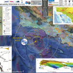
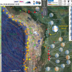
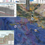
Well well.
There was lots of interest in this M 5.3 earthquake offshore of Ventura/Los Angeles, justifiably so. Southern California is earthquake country.

Here is an update. There was lots of information that I was trying to incorporate and I needed an additional report to cover some of this material. That being said, there is still some mystery about this earthquake. My favored interpretation is that this EQ was a left-lateral strike-slip earthquake. There is still room to interpret this as a right-lateral strike-slip (llss) earthquake however.

Below I have prepared some figures that provide additional information that helps us learn about the faulting and basin development in the CA Borderlands here. There is lots of work that has been done here and this is far from a comprehensive analysis.

As I mentioned before (here is my initial Earthquake Report for this EQ), due to the big bend in the San Andreas fault (SAF) in southern CA, there is evidence for compression in the form of thrust faults and uplifted mountains (e.g. Sierra Madre fault and the San Gabriel Mtns). One of these thrust faults (which may also have some strike-slip motion) is the Hollywood fault (recently highlighted by the recent work by the CA Geological Survey).

Also part of the development of the SAF involved the clockwise rotation of a crustal block where the Transverse Ranges are (the mtns to the north of Ventura/Santa Barbara). Along the southern boundary of the Transverse Ranges formed left-lateral strike slip faults. The Santa Cruz Island fault just happens to be a left-lateral strike-slip fault.

The CA Borderlands is a complex region of faulting, inheriting structures from the Tertiary, overprinted by modern tectonics and everything in between. The Hollywood fault trends towards (and turns into?) the Malibu Coast fault, which may turn into the Santa Cruz Island fault (SCIF), a vertical left-lateral strike-slip fault (but may have some vertical motion on it, based upon offsets in vertical uplift rates from marine terrace profiles).

Schindler used seismic reflection profiles in the Santa Cruz Basin area to interpret the tectonic history here. I placed the faults interpreted by them as orange lines in the interpretive poster (labeled as the Ferrelo fault and the East Santa Cruz (ECS) Basin fault system). The ESCBFS is a thrust fault system, with possible oblique motion (strike-slip). My initial interpretation was that this M 5.3 was a llss earthquake associated with this fault. There are some interesting problems that arise considering this fault. To the south, the fault is oriented similar to the San Clemente fault (which may have had a M 5.5 right-lateral strike-slip (rlss) earthquake on 1981.09.04). Due to this, the simple interpretation is that the ESCBFS is right lateral oblique at the southern part of the Santa Cruz Basin. However, along the northern boundary of this basin, the ESCBFS rotates to an east-west strike (orientation). The simple interpretation would be that this part of the fault system would be llss, similar to the SCIF. So, clearly, things are not so simple here. See the Chaytor et al. (2008) figure below.

That being said, if this M 5.3 earthquake was on an east-west fault, it would be llss. There is no evidence for a north-south oriented fault on the western boundary of the Santa Cruz Basin (see Schindler (2007) seismic profile below), supporting the left-lateral interpretation.

Below is my interpretive poster for this earthquake

I plot the seismicity from the past month, with color representing depth and diameter representing magnitude (see legend). I include earthquake epicenters from 1918-2018 with magnitudes M ≥ 4.5.

I plot the USGS fault plane solutions (moment tensors in blue and focal mechanisms in orange) for the M 5.3 earthquake, in addition to some relevant historic earthquakes (including the 1971 Sylmar and 1994 Northridge earthquakes, as evidence for the compression in the region).

  • I placed a moment tensor / focal mechanism legend on the poster. There is more material from the USGS web sites about moment tensors and focal mechanisms (the beach ball symbols). Both moment tensors and focal mechanisms are solutions to seismologic data that reveal two possible interpretations for fault orientation and sense of motion. One must use other information, like the regional tectonics, to interpret which of the two possibilities is more likely.
  • I also include the shaking intensity contours on the map. These use the Modified Mercalli Intensity Scale (MMI; see the legend on the map). This is based upon a computer model estimate of ground motions, different from the “Did You Feel It?” estimate of ground motions that is actually based on real observations. The MMI is a qualitative measure of shaking intensity. More on the MMI scale can be found here and here. This is based upon a computer model estimate of ground motions, different from the “Did You Feel It?” estimate of ground motions that is actually based on real observations.
  • I include the slab contours plotted (Hayes et al., 2012), which are contours that represent the depth to the subduction zone fault. These are mostly based upon seismicity. The depths of the earthquakes have considerable error and do not all occur along the subduction zone faults, so these slab contours are simply the best estimate for the location of the fault.
  • I include some inset figures.

  • In the upper left corner is a cross section from Shaw and Suppe (1994). This cross section location is shown on the interpretive poster as a blue line labeled X-Y. This cross section (from interpretations of offshore seismic reflection profiles) shows the major player here is a thrust fault, the Channel Islands Thrust. Note the SCIF is also shown to rip right through Santa Cruz Island.
  • In the upper right corner is a map that shows the area of this fault ramp of the Channel Islands Thrust (Shaw and Suppe, 1994). Note that this fault ramp area is also shown on the interpretive poster, outlined in light orange.
  • In the center left is a figure from Fuis et al. (2001) that shows a block diagram revealing how the north-south convergence (from the bend in the San Andreas) is accommodated by thrust/reverse faults. The Sierra Madre fault is also labeled on the interpretive poster. A recent earthquake in La Habra is an example of this north-south compression. Here are my report and report update for this M 5.1 La Habra earthquake.
  • In the lower left corner is a seismic reflection profile from Schindler (2007), from her Master’s Thesis. The profile A-A’ is shown on the map as a green line labeled A-A’. Note that there is no faulting on the western boundary of the Santa Cruz Basin. When I first looked at this section, I thought that the ESCBFS were either normal (extensional) or strike-slip faults. After reading her thesis, I learned that these faults did have normal offset (in the Miocene Epoch, part of the Tertiary Period), but have been reactivated as thrust faults in post-Miocene time. The San Clemente fault (labeled on the interpretive poster) turns into the Santa Cruz-Catalina Ridge fault (labeled on this cross section).
  • In the lower right corner is a figure that shows how these faults interact in a complicated manner (Sorlien et al., 2006). This figure was prepared after they interpreted seismic reflection profile data. The upper panel is a low-angle oblique view of the faults in 3-D view. The lower two panels are the cross sections B-B’ and E-E’ (also shown on the interpretive poster as orange lines). These cross sections show how the Malibu Coast fault is more deeply dipping (more close to vertical) compared to the Santa Monica-Dume fault (a shallow dipping thrust fault). Both of these faults appear to join in some way near the coast, where they turn into the Hollywood fault. There are probably some inaccuracies in how I am interpreting how these faults interact beyond the limit of the figures I present here.


  • Here is the same map including the magnetic anomaly data (the red and blue shades).


USGS Earthquake Pages

Some Relevant Discussion and Figures

  • Here is a map that shows where the seismic profile was acquired (Shaw and SUppe, 1994).

  • Epicenters from an earthquake swarm in 1984 (Henyey and Teng, 1985) define the active axial surface (A) of the Offshore Oak Ridge trend. Single-event (C and D) and composite (E and F) focal mechanism solutions from the 1984 seismicity have gentle north dipping (C, D, and E) and horizontal (F) nodal planes (Henyey and Teng, 1985) consistent with folding through the active axial surfaces by bedding parallel slip (see Figure 10B). Cross section traces: X-X’ (Fig. 7); X-Y (Fig. 11). SCIF = Santa Cruz Island fault.

  • Here is the cross section. The upper panel shows the modern configuration and the lower panel shows their interpretation during the Tertiary (Shaw and Suppe, 1994).

  • A balanced geologic cross section across the eastern Santa Barbara Channel and Santa Cruz Island combines subsurface seismic reflection and well-log data (the section trace is in Figs. 1 and 10A). The Channel Islands thrust ramps beneath the Offshore Oak Ridge trend and approaches the surface south of Santa Cruz Island. The kink-band width (A-A’) of the Offshore Oak Ridge trend represents dip slip on the underlying Channel Islands thrust. The shallow fold and fault geometry along the Offshore Oak Ridge and Blue Bottle trends is depicted in Figure 7. Strike-slip motion out of the section plane may occur on the Santa Cruz Island fault; however, moderate displacements on this fault should not significantly effect our area balance and restoration, because the strike-slip fault trace is perpendicular to the section plane (Fig. 10A). SCIF = Santa Cruz Island fault. Horizontal equals vertical scale.

  • For background, here is a timeline for the tectonics along the Pacific-North America plate boundary (Schindler, 2007). The Transverse Ranges block is shown as a green bleb labeled WTR. Note how this block is rotating in a clockwise fasion, and see that there are strike-slip faults that form along the block edge to accommodate this rotation.

  • A simple tectonic model of the evolution of the Pacific-North American plate boundary that includes the Inner and Outer Borderland (IB, OB) and rotation of the western Transverse Ranges (WTR) province (from Nicholson et al, 1994). The model assumes a constant rate and direction of Pacific plate motion and constant rate of western Transverse Ranges rotation. As each partially subducted microplate is captured by the Pacific plate (Monterey, ~19 Ma; Arguello, ~17.5 Ma; Guadalupe and Magdalena, ~12 Ma), this results in a transfer of part of the over-riding North American upper plate to the Pacific plate. The fine gray lines provide a reference grid fixed to North America. ArP-Arguello plate; GP-Guadalupe plate; MtP-Monterey plate; SG-San Gabriel block; JdFP-Juan de Fuca plate; SLB-San Lucia Bank; SMB-Santa Maria basin; SB-southern Borderland;T-AFTosco- Arbreojos fault; MP-Magdalena plate. Red areas are regions of transtension; Purple areas are captured or soon to be captured microplates.

  • Here is the seismic reflection profile from Schindler (2010).

  • Regional seismic line WC82-108 showing the ~50 km wide Santa Rosa Ridge anticlinorium. Parallel bedding of pre-Pliocene strata indicates that this anticlinal structure formed post Miocene. The Cretaceous-Paleogene sedimentary rocks are eroded by the early Miocene unconformity (green) and truncate against basement (black arrows). Mapped reference horizons and faults are shown in color and in black, respectively.

  • This is a fantastic low-angle oblique view of the topography and bathymetry of this region (and the Santa Cruz Basin) from Schindler (2010). The figure caption is embedded in the figure.

  • This is the figure from Schindler (2010) that shows the geometry of the ESCBFS and Ferrlo faults. Red shows the upper part of the faults. These faults dip to the north, northeast, and east.

  • A map view of 3D fault surfaces surrounding Santa Cruz basin in the northern Borderland. Depths down-dip along fault surfaces are shown as changing colors at even kilometer levels. The ESCB fault system is observed to be a gently east- to northeast-dipping, right stepping, en echelon reactivated reverse or oblique-reverse fault that bends to become more northerly dipping as it approaches Santa Cruz Island.

  • There has been lots of work here. Jason Chaytor (now at USGS in Woods Hole) worked on submerged marine terraces in this region. These marine terraces were formed when sea level was lower and are a result of erosion from ocean waves at that time. Dr. Chaytor used radiometric ages and sea level curve data to evaluate the tectonic uplift in the region. Here is a map that shows Jason’s interpretation of the seismic profiles for this region (same seismic data used by Schindler).

  • Preliminary map of geologic structures currently mapped using multichannel sparker, and recently released WesternGeco multichannel seismic-reflection profiles (modified from Chaytor, 2006). SCIF—Santa Cruz Island fault.

Geologic Fundamentals

  • For more on the graphical representation of moment tensors and focal mechnisms, check this IRIS video out:
  • Here is a fantastic infographic from Frisch et al. (2011). This figure shows some examples of earthquakes in different plate tectonic settings, and what their fault plane solutions are. There is a cross section showing these focal mechanisms for a thrust or reverse earthquake. The upper right corner includes my favorite figure of all time. This shows the first motion (up or down) for each of the four quadrants. This figure also shows how the amplitude of the seismic waves are greatest (generally) in the middle of the quadrant and decrease to zero at the nodal planes (the boundary of each quadrant).

  • There are three types of earthquakes, strike-slip, compressional (reverse or thrust, depending upon the dip of the fault), and extensional (normal). Here is are some animations of these three types of earthquake faults. The following three animations are from IRIS.
  • Strike Slip:

    Compressional:

    Extensional:

Social Media

    References:

    Basic & General References

  • Frisch, W., Meschede, M., Blakey, R., 2011. Plate Tectonics, Springer-Verlag, London, 213 pp.
  • Hayes, G., 2018, Slab2 – A Comprehensive Subduction Zone Geometry Model: U.S. Geological Survey data release, https://doi.org/10.5066/F7PV6JNV.
  • Holt, W. E., C. Kreemer, A. J. Haines, L. Estey, C. Meertens, G. Blewitt, and D. Lavallee (2005), Project helps constrain continental dynamics and seismic hazards, Eos Trans. AGU, 86(41), 383–387, , https://doi.org/10.1029/2005EO410002. /li>
  • Jessee, M.A.N., Hamburger, M. W., Allstadt, K., Wald, D. J., Robeson, S. M., Tanyas, H., et al. (2018). A global empirical model for near-real-time assessment of seismically induced landslides. Journal of Geophysical Research: Earth Surface, 123, 1835–1859. https://doi.org/10.1029/2017JF004494
  • Kreemer, C., J. Haines, W. Holt, G. Blewitt, and D. Lavallee (2000), On the determination of a global strain rate model, Geophys. J. Int., 52(10), 765–770.
  • Kreemer, C., W. E. Holt, and A. J. Haines (2003), An integrated global model of present-day plate motions and plate boundary deformation, Geophys. J. Int., 154(1), 8–34, , https://doi.org/10.1046/j.1365-246X.2003.01917.x.
  • Kreemer, C., G. Blewitt, E.C. Klein, 2014. A geodetic plate motion and Global Strain Rate Model in Geochemistry, Geophysics, Geosystems, v. 15, p. 3849-3889, https://doi.org/10.1002/2014GC005407.
  • Meyer, B., Saltus, R., Chulliat, a., 2017. EMAG2: Earth Magnetic Anomaly Grid (2-arc-minute resolution) Version 3. National Centers for Environmental Information, NOAA. Model. https://doi.org/10.7289/V5H70CVX
  • Müller, R.D., Sdrolias, M., Gaina, C. and Roest, W.R., 2008, Age spreading rates and spreading asymmetry of the world’s ocean crust in Geochemistry, Geophysics, Geosystems, 9, Q04006, https://doi.org/10.1029/2007GC001743
  • Pagani,M. , J. Garcia-Pelaez, R. Gee, K. Johnson, V. Poggi, R. Styron, G. Weatherill, M. Simionato, D. Viganò, L. Danciu, D. Monelli (2018). Global Earthquake Model (GEM) Seismic Hazard Map (version 2018.1 – December 2018), DOI: 10.13117/GEM-GLOBAL-SEISMIC-HAZARD-MAP-2018.1
  • Silva, V ., D Amo-Oduro, A Calderon, J Dabbeek, V Despotaki, L Martins, A Rao, M Simionato, D Viganò, C Yepes, A Acevedo, N Horspool, H Crowley, K Jaiswal, M Journeay, M Pittore, 2018. Global Earthquake Model (GEM) Seismic Risk Map (version 2018.1). https://doi.org/10.13117/GEM-GLOBAL-SEISMIC-RISK-MAP-2018.1
  • Zhu, J., Baise, L. G., Thompson, E. M., 2017, An Updated Geospatial Liquefaction Model for Global Application, Bulletin of the Seismological Society of America, 107, p 1365-1385, https://doi.org/0.1785/0120160198
  • Specific References

  • Chaytor, J.D., Goldfinger, C., Meiner, M.A., Huftile, G.J., Romsost, C.G., Legg, M.R., 2008. Measuring vertical tectonic motion at the intersection of the Santa Cruz–Catalina Ridge and Northern Channel Islands platform, California Continental Borderland, using submerged paleoshorelines in GSA Bulletin, v. 120, no. 7/8, p. 1053-1071, doi: 10.1130/B26316.1
  • Du, X., Hendy, I., Schimmelmann, 2018. A 9000-year flood history for Southern California: A revised stratigraphy of varved sediments in Santa Barbara Basin in Marine Geology, v. 397, p. 29-42, https://doi.org/10.1016/j.margeo.2017.11.014
  • Fuis, G.S., Ryberg, T., Godfrey, N.J., Okaya, D.A., Murphy, J.M., 2001. Crustal structure and tectonics from the Los Angeles basin to the Mojave Desert, southern California in Geology, v. 29, no. 1, p. 15-18
  • Legg, M. R., M. D. Kohler, N. Shintaku, and D. S. Weeraratne, 2015. Highresolution mapping of two large-scale transpressional fault zones in the California Continental Borderland: Santa Cruz-Catalina Ridge and Ferrelo faults, J. Geophys. Res. Earth Surf., 120, 915–942, doi:10.1002/2014JF003322.
  • Pinter, N., Lueddecke, S.B., Keller, E.A., Simmons, K.R., 1998. Late Quaternary slip on the Santa Cruz Island fault, California in GSA Bulletin, v. 110, no. 6, p. 711-722
  • Pinter, N., Johns, B., Little, B., Vestal, W.D., 2001. Fault-Related Folding in California’s Northern Channel Islands Documented by Rapid-Static GPS Positioning in GSA Today, May, 2001
  • Schindler, C.S., 2010. 3D Fault Geometry and Basin Evolution in the Northern Continental Borderland Offshore Southern California Catherine Sarah Schindler, B.S. A Thesis Submitted to the Department of Physics and Geology California State University Bakersfield In Partial Fulfillment for the Degree of Masters of Science in Geology
  • Shaw, J.H., Suppe, J., 1994. Active faulting and growth folding in the eastern Santa Barbara Channel, California in GSA Bulletin, v. 106, p. 607-626
  • Wallace, Robert E., ed., 1990, The San Andreas fault system, California: U.S. Geological Survey Professional Paper 1515, 283 p. [https://pubs.er.usgs.gov/publication/pp1515].

Return to the Earthquake Reports page.

Earthquake Report: Channel Islands

I was finally getting around to writing a report for the deep Bolivia earthquake (Bolivia report here), when a M 5.3 earthquake struck offshore of the channel islands (south of Santa Cruz Island, west of Los Angeles). As is typical when an earthquake hits a populated region in the USA, the USGS websites stopped working (for the earthquakes in South America I was researching). After about half an hour or so, the websites started working again (the M 5.3 earthquake website never had a problem).

The Los Angeles region is dominated by the tectonics associated with the North America – Pacific transform plate boundary system of the San Andreas fault (SAF). The SAF accommodates the majority of plate motion between these two plates. There are sister faults where some of the plate boundary motion also goes. This plate boundary extends from the Pacific Ocean eastwards to Utah (the Wasatch fault system).

The SAF is considered a “mature” strike-slip fault because it is straight along most of the system. We think that strike-slip faults start out as smaller faults that develop as tectonic strain enters a region that is different from prior strain. As time passes, these smaller faults join each other, to align with the great circle aligned to the euler pole (the axis of rotation for plates).

The SAF does bend in some places, most notably in southern CA. This bend creates complexities in the fault, but also results in north-south compression (and thrust faults) forming the Transverse Ranges north of the LA Basin. Recent work by the California Geological Survey has been focusing on these thrust faults as they strike (trend) through Hollywood. These thrust faults are oriented east-west.

There are also additional faults offshore of LA in what is called the borderlands. Many of these faults are sub-parallel to the SAF. The best example is the Newport Inglewood fault (NIF), the locus of the 1933 Long Beach Earthquake. This fault is offshore, but also extends onshore. The NIF is generally a northwest-southeast striking right lateral strike-slip fault just like the SAF.

Some of the east-west faults also extend offshore. Onshore, they are generally thrust faults, but less is known about what they do offshore (i.e. they could have some strike-slip motion too).

Today’s earthquake happened south of Santa Catalina Island, where there is a major fault system that runs through the island: the Santa Cruz Island fault. This fault is mostly a left-lateral strike-slip fault, with a small portion of reverse (compression) motion (Pinter et al, 1998, 2001).
To the north of SC Island, is the Santa Barbara Basin, an oceanic basin that preserves an excellent record of flood and earthquake triggered sedimentary deposits.

If today’s M 5.3 is possibly related to the faults that form the Santa Cruz Basin. I provide some maps of this region below the interpretive poster. Based upon the work conducted by Schindler for their MS Thesis, Today’s earthquake appears associated with the East Santa Cruz Basin fault system (supporting that this was a left-lateral strike-slip earthquake). This is not included in the USGS active fault and fold database, but today’s earthquake suggests that it could be added.

These sedimentary basins are most likely formed from extension when the orientation of strike slip faults is not parallel to the plate motion. These are called “pull apart” basins and are a result of “transtension.” Do an internet search for more about transtension and how pull apart basins can form.

After one reads this report, check out the update here.

Below is my interpretive poster for this earthquake

I plot the seismicity from the past month, with color representing depth and diameter representing magnitude (see legend). I include earthquake epicenters from 1918-2018 with magnitudes M ≥ 4.5.

I plot the USGS fault plane solutions (moment tensors in blue and focal mechanisms in orange) for the M 5.3 earthquake, in addition to some relevant historic earthquakes.

  • I placed a moment tensor / focal mechanism legend on the poster. There is more material from the USGS web sites about moment tensors and focal mechanisms (the beach ball symbols). Both moment tensors and focal mechanisms are solutions to seismologic data that reveal two possible interpretations for fault orientation and sense of motion. One must use other information, like the regional tectonics, to interpret which of the two possibilities is more likely.
  • I also include the shaking intensity contours on the map. These use the Modified Mercalli Intensity Scale (MMI; see the legend on the map). This is based upon a computer model estimate of ground motions, different from the “Did You Feel It?” estimate of ground motions that is actually based on real observations. The MMI is a qualitative measure of shaking intensity. More on the MMI scale can be found here and here. This is based upon a computer model estimate of ground motions, different from the “Did You Feel It?” estimate of ground motions that is actually based on real observations.
  • I include some inset figures.

  • On the right side of the poster are figures from Wallace (1990) and show the main faults associated with the SAF system. I place a blue star in the general location of today’s earthquake (as also in other places on this poster).
  • To the upper left of the Wallace SAF map for California is a figure also from Wallace (1990) that shows more details, including elevation information (color = height or depth).
  • To the lower left of the Wallace SAF map for CA is a figure that shows the high resolution bathymetry (seafloor shape) for the Santa Cruz Basin.
  • In the upper left corner is a seismotectonic map of the CA Borderlands (Legg et al., 2015). They show faults and their sense of motion. There are also focal mechanisms for historic earthquakes.
  • In the lower left corner is a larger scale map of this region, showing the faults as mapped by Schindler (2007).


USGS Earthquake Pages

Some Relevant Discussion and Figures

  • Here is the figure showing the evolution of the SAF since its inception about 29 Ma. I include the USGS figure caption below as a blockquote.
  • EVOLUTION OF THE SAN ANDREAS FAULT.
    This series of block diagrams shows how the subduction zone along the west coast of North America transformed into the San Andreas Fault from 30 million years ago to the present. Starting at 30 million years ago, the westward- moving North American Plate began to override the spreading ridge between the Farallon Plate and the Pacific Plate. This action divided the Farallon Plate into two smaller plates, the northern Juan de Fuca Plate (JdFP) and the southern Cocos Plate (CP). By 20 million years ago, two triple junctions began to migrate north and south along the western margin of the West Coast. (Triple junctions are intersections between three tectonic plates; shown as red triangles in the diagrams.) The change in plate configuration as the North American Plate began to encounter the Pacific Plate resulted in the formation of the San Andreas Fault. The northern Mendicino Triple Junction (M) migrated through the San Francisco Bay region roughly 12 to 5 million years ago and is presently located off the coast of northern California, roughly midway between San Francisco (SF) and Seattle (S). The Mendicino Triple Junction represents the intersection of the North American, Pacific, and Juan de Fuca Plates. The southern Rivera Triple Junction (R) is presently located in the Pacific Ocean between Baja California (BC) and Manzanillo, Mexico (MZ). Evidence of the migration of the Mendicino Triple Junction northward through the San Francisco Bay region is preserved as a series of volcanic centers that grow progressively younger toward the north. Volcanic rocks in the Hollister region are roughly 12 million years old whereas the volcanic rocks in the Sonoma-Clear Lake region north of San Francisco Bay range from only few million to as little as 10,000 years old. Both of these volcanic areas and older volcanic rocks in the region are offset by the modern regional fault system. (Image modified after original illustration by Irwin, 1990 and Stoffer, 2006.)

  • Here is a map that shows the shaking potential for earthquakes in CA. This comes from the state of California here. Note how Santa Cruz Island has an increased chance of hazard due to the Santa Cruz Island fault.

  • Earthquake shaking hazards are calculated by projecting earthquake rates based on earthquake history and fault slip rates, the same data used for calculating earthquake probabilities. New fault parameters have been developed for these calculations and are included in the report of the Working Group on California Earthquake Probabilities. Calculations of earthquake shaking hazard for California are part of a cooperative project between USGS and CGS, and are part of the National Seismic Hazard Maps. CGS Map Sheet 48 (revised 2008) shows potential seismic shaking based on National Seismic Hazard Map calculations plus amplification of seismic shaking due to the near surface soils.

  • Here is a map that shows the tectonic provides in this region (Legg et al. (2015). While the region inherits topography and geologic structures from past tectonic regimes, the dominant tectonic control here is currently the North America – Pacific plate boundary.

  • Map of the California Continental Borderland showing major tectonic features and moderate earthquake locations (M >5.5). The dashed box shows area of this study. The large arrows show relative plate motions for the Pacific-North America transform fault boundary (~N40° ± 2°W; RM2 and PA-1 [Plattner et al., 2007]). BP = Banning Pass, CH = Chino Hills, CP = Cajon Pass, LA = Los Angeles, PS = Palm Springs, V = Ventura, ESC = Santa Cruz Basin, ESCBZ = East Santa Cruz Basin fault zone, SCI = Santa Catalina Island, SCL = San Clemente Island, SMB = Santa Monica Basin, and SNI = San Nicolas Island. Base map from GeoMapApp/Global Multi-Resolution Topography (GMRT) [Ryan et al., 2009].

  • This shows the timeline of what has controlled the tectonics in this region (Legg et al., 2015).

  • Chronology of major Cenozoic events in the Southern California region (after Wright [1991] and Legg and Kamerling [2012]). Intensity of tectonic deformation is represented by the curve. Local (Los Angeles Basin) biostratigraphic zonation is shown. The slanted labels for Neogene stages represent the time-transgressive nature of these boundaries.

  • Here is the figure with more details about the tectonic interpretation of the area (Legg et al., 2015)

  • Map showing bathymetry, Quaternary faults, and recent seismicity in the Outer Borderland. Fault locations are based on the high-resolution bathymetry, available high-resolution seismic reflection profiles, and published fault maps [cf. California Geological Survey (CGS), 2010]. The red symbols show magnitude-scaled (M>4) epicenters for seismicity recorded for the period of 1932 to 2013. Seismicity data and focal mechanisms are derived from the Southern California Seismograph Network catalogs, National Earthquake Information Center [2012–2013], and Legg [1980]. Focal mechanism event numbers correspond to Table S2 in the supporting information. The black rectangle shows location of Figure 10. The light blue lines show tracklines of multichannel seismic profiles—the labeled white profiles are shown in Figures 12 (124) and 13 (108 and 126).

  • Here is the summary figure from Legg et al. (2015). This helps us put these faults systems into context.

  • Map showing major active tectonic elements of the northern part of the California Continental Borderland. Major active (Quaternary) faults are shown in red (SAF = San Andreas fault, ABF = Agua Blanca fault, SCF = San Clemente fault, and SCCR = Santa Cruz-Catalina Ridge, Ferrelo). Major strike-slip offsets are shown by shaded areas with estimated displacement (EK = Emery Knoll crater; Tanner Basin near DB = Dall Bank; and SDT = San Diego Trough, small pull-apart near Catalina). Other symbols show oblique fault character including transpressional restraining bends (CAT = Santa Catalina Island, CB = Cortes Bank, and TB = Tanner Bank), uplifts (SRI = Santa Rosa Island, SCz = Santa Cruz Island, SNI = San Nicolas Island, CB = Cortes Bank, TB = Tanner Bank, and SBM = San Bernardino Mountains), and transtensional pull-apart basins (SD = San Diego, ENS = Ensenada, SCB = San Clemente Basin, and SIB = San Isidro Basin). The large arrows show Pacific-North America relative plate motions with the blue dashed line (PAC-NAM) along a small circle for the RM2 [Minster and Jordan, 1978] plate motions model through San Clemente Island (SCL). Boundary between the Inner and Outer Borderland follows the East Santa Cruz Basin fault zone (dotted line; modified from Schindler [2010] and De Hoogh [2012]). Holocene volcanoes exist along the coast (SQ= San Quintín) and within the Gulf of California Rift (CP = Cerro Prieto and Obsidian Buttes, Salton Trough). Dates show year of earthquakes with mapped focal mechanisms (see Table S2 in the supporting information). SB = Santa Barbara, LA = Los Angeles, and PS = Palm Springs.

  • The Santa Barbara Basin to the north has an excellent Holocene record of floods and earthquakes (Du et al., 2018). Here is a plot showing the ages of possible earthquake triggered turbidites (submarine landslide deposits) from the Santa Barbara Basin.

  • Probability density functions (PDFs) for the 19 turbidites (olive layers) in core MV0811-14JC and core SPR090106KC in Santa Barbara Basin generated from Bacon 2.2. Brackets show 95% confidence intervals. Estimate emergence times of the Newport-Inglewood Fault (Leeper et al., 2017) in pink, Ventura- Pitas Point Fault (Rockwell et al., 2016) in green, Ventura blind thrust fault (McAuliffe et al., 2015) in purple, Compton Thrust Fault (Leon et al., 2009) in yellow and the Goleta Slide Complex (Fisher et al., 2005)in gray. Age of slumped material in 14JC is indicated by wavy texture. (For interpretation of the references to colour in this figure legend, the reader is referred to the web version of this article.)

  • As I mentioned, there is some uplift associated with compression along the Santa Cruz Island fault (Pinter et al., 2001). This plot shows uplift across the region in the form of uplifted marine terraces. This plot assumes these marine terraces were formed at the same time, so if there were no differential tectonic uplift, these lines would be horizontal.

  • Cross-sectional profile A-B-C on Santa Rosa Island (see Fig. 3) showing corrected terrace elevations. SRIF shows the locations of the Santa Rosa Island fault. Error bars are the sum of the ±1 s uncertainties in wave-cut platform slope and the GPS measurement errors. Note the change in vertical exaggeration between the lower and upper plots. The green curve was qualitatively fit to the T2 data in order to create the smoothest possible curve that conforms to all points; other curves are scaled versions of the T2 curve. Point spacing is too coarse and error bars too large on the other levels to show deformation details, but the scaled curves show that every measured point is consistent with the pattern measured on T2.

  • This is a diagram that shows how a pull apart basin might form (Wu et al., 2009).

  • General characteristics of a pull-apart basin in a dextral side-stepping fault system. The pull-apart basin is defined to develop in pure strike-slip when alpha = 0 degrees and in transtension when 0 degrees < alpha 45 degrees.

  • This figure shows the results of modeling in clay, showing a pull apart basin form (Wu et al., 2009).

  • Plan view evolution of transtensional pull-apart basin model illustrated with: (a) time-lapse overhead photography; and (b) fault interpretation and incremental basin subsidence calculated from differential laser scans. Initial and final baseplate geometry shown with dashed lines; (c) basin topography at end of experiment.

Geologic Fundamentals

  • For more on the graphical representation of moment tensors and focal mechnisms, check this IRIS video out:
  • Here is a fantastic infographic from Frisch et al. (2011). This figure shows some examples of earthquakes in different plate tectonic settings, and what their fault plane solutions are. There is a cross section showing these focal mechanisms for a thrust or reverse earthquake. The upper right corner includes my favorite figure of all time. This shows the first motion (up or down) for each of the four quadrants. This figure also shows how the amplitude of the seismic waves are greatest (generally) in the middle of the quadrant and decrease to zero at the nodal planes (the boundary of each quadrant).

  • There are three types of earthquakes, strike-slip, compressional (reverse or thrust, depending upon the dip of the fault), and extensional (normal). Here is are some animations of these three types of earthquake faults. The following three animations are from IRIS.
  • Strike Slip:

    Compressional:

    Extensional:

Social Media

    References:

    Basic & General References

  • Frisch, W., Meschede, M., Blakey, R., 2011. Plate Tectonics, Springer-Verlag, London, 213 pp.
  • Hayes, G., 2018, Slab2 – A Comprehensive Subduction Zone Geometry Model: U.S. Geological Survey data release, https://doi.org/10.5066/F7PV6JNV.
  • Holt, W. E., C. Kreemer, A. J. Haines, L. Estey, C. Meertens, G. Blewitt, and D. Lavallee (2005), Project helps constrain continental dynamics and seismic hazards, Eos Trans. AGU, 86(41), 383–387, , https://doi.org/10.1029/2005EO410002. /li>
  • Jessee, M.A.N., Hamburger, M. W., Allstadt, K., Wald, D. J., Robeson, S. M., Tanyas, H., et al. (2018). A global empirical model for near-real-time assessment of seismically induced landslides. Journal of Geophysical Research: Earth Surface, 123, 1835–1859. https://doi.org/10.1029/2017JF004494
  • Kreemer, C., J. Haines, W. Holt, G. Blewitt, and D. Lavallee (2000), On the determination of a global strain rate model, Geophys. J. Int., 52(10), 765–770.
  • Kreemer, C., W. E. Holt, and A. J. Haines (2003), An integrated global model of present-day plate motions and plate boundary deformation, Geophys. J. Int., 154(1), 8–34, , https://doi.org/10.1046/j.1365-246X.2003.01917.x.
  • Kreemer, C., G. Blewitt, E.C. Klein, 2014. A geodetic plate motion and Global Strain Rate Model in Geochemistry, Geophysics, Geosystems, v. 15, p. 3849-3889, https://doi.org/10.1002/2014GC005407.
  • Meyer, B., Saltus, R., Chulliat, a., 2017. EMAG2: Earth Magnetic Anomaly Grid (2-arc-minute resolution) Version 3. National Centers for Environmental Information, NOAA. Model. https://doi.org/10.7289/V5H70CVX
  • Müller, R.D., Sdrolias, M., Gaina, C. and Roest, W.R., 2008, Age spreading rates and spreading asymmetry of the world’s ocean crust in Geochemistry, Geophysics, Geosystems, 9, Q04006, https://doi.org/10.1029/2007GC001743
  • Pagani,M. , J. Garcia-Pelaez, R. Gee, K. Johnson, V. Poggi, R. Styron, G. Weatherill, M. Simionato, D. Viganò, L. Danciu, D. Monelli (2018). Global Earthquake Model (GEM) Seismic Hazard Map (version 2018.1 – December 2018), DOI: 10.13117/GEM-GLOBAL-SEISMIC-HAZARD-MAP-2018.1
  • Silva, V ., D Amo-Oduro, A Calderon, J Dabbeek, V Despotaki, L Martins, A Rao, M Simionato, D Viganò, C Yepes, A Acevedo, N Horspool, H Crowley, K Jaiswal, M Journeay, M Pittore, 2018. Global Earthquake Model (GEM) Seismic Risk Map (version 2018.1). https://doi.org/10.13117/GEM-GLOBAL-SEISMIC-RISK-MAP-2018.1
  • Zhu, J., Baise, L. G., Thompson, E. M., 2017, An Updated Geospatial Liquefaction Model for Global Application, Bulletin of the Seismological Society of America, 107, p 1365-1385, https://doi.org/0.1785/0120160198
  • Specific References

  • Du, X., Hendy, I., Schimmelmann, 2018. A 9000-year flood history for Southern California: A revised stratigraphy of varved sediments in Santa Barbara Basin in Marine Geology, v. 397, p. 29-42, https://doi.org/10.1016/j.margeo.2017.11.014
  • Legg, M. R., M. D. Kohler, N. Shintaku, and D. S. Weeraratne, 2015. Highresolution mapping of two large-scale transpressional fault zones in the California Continental Borderland: Santa Cruz-Catalina Ridge and Ferrelo faults, J. Geophys. Res. Earth Surf., 120, 915–942, doi:10.1002/2014JF003322.
  • Pinter, N., Lueddecke, S.B., Keller, E.A., Simmons, K.R., 1998. Late Quaternary slip on the Santa Cruz Island fault, California in GSA Bulletin, v. 110, no. 6, p. 711-722
  • Pinter, N., Johns, B., Little, B., Vestal, W.D., 2001. Fault-Related Folding in California’s Northern Channel Islands Documented by Rapid-Static GPS Positioning in GSA Today, May, 2001
  • Schindler, C.S., 2010. 3D Fault Geometry and Basin Evolution in the Northern Continental Borderland Offshore Southern California Catherine Sarah Schindler, B.S. A Thesis Submitted to the Department of Physics and Geology California State University Bakersfield In Partial Fulfillment for the Degree of Masters of Science in Geology
  • Wallace, Robert E., ed., 1990, The San Andreas fault system, California: U.S. Geological Survey Professional Paper 1515, 283 p. [https://pubs.er.usgs.gov/publication/pp1515].

Return to the Earthquake Reports page.

Earthquake Report: Bolivia!

A couple days ago there was a deep focus earthquake in the downgoing Nazca plate deep beneath Bolivia. This earthquake has an hypocentral depth of 562 km (~350 miles).
We are still unsure what causes an earthquake at such great a depth. The majority of earthquakes happen at shallower depths, caused largely by the frictional between differently moving plates or crustal blocks (where earth materials like the crust behave with brittle behavior and not elastic behavior). Some of these shallow earthquakes are also due to internal deformation within plates or crustal blocks.
As plates dive into the Earth at subduction zones, they undergo a variety of changes (temperature, pressure, stress). However, because people cannot directly observe what is happening at these depths, we must rely on inferences, laboratory analogs, and other indirect methods to estimate what is going on.
So, we don’t really know what causes earthquakes at the depth of this Bolivia M 6.8 earthquake. Below is a review of possible explanations as provided by Thorne Lay (UC Santa Cruz) in an interview in response to the 2013 M 8.3 Okhotsk Earthquake.
There are lots of examples in this region of South America for deep earthquakes. They are all extensional (normal fault) earthquakes.

One option could be “fluid-assisted faulting,” in which water is released from minerals as they change phases during faulting, thus lubricating the plates, Lay says.
But although this is a common mechanism for earthquakes between 70 and 400 kilometers deep, it’s unlikely to be the cause of this quake because the plate is significantly dewatered by the time it reaches 400 kilometers deep. Minerals releasing carbon dioxide as they are compacted could provide an alternative fluid to lubricate the fault, he says, much like water does at shallower depths.
And another possibility is that a transition in mineral form from low-pressure polymorphs (the form in which a mineral is stable at the surface) to high-pressure polymorphs (a denser form of a mineral that is stable at greater depths), gives the fault a start. According to this model, the plate subducts too quickly for the mineral to slowly transition to its denser form. The mineral will reach depths greater than where it is normally stable, and thus the transformation may be a catastrophic process, causing a jolt at 600 kilometers, which would allow for movement along the fault, Lay says.

There have been a number of deep earthquakes globally in the past several years. These include the 2013 M 8.3 in the Sea of Okhtosk, the 2015 M 7.8 along the Izu-Bonin Arc, and several along the central Andes. I present some interpretive posters for these earthquakes below.

Below is my interpretive poster for this earthquake

I plot the seismicity from the past month, with color representing depth and diameter representing magnitude (see legend). I include earthquake epicenters from 1918-2018 with magnitudes M ≥ 6.5.
I plot the USGS fault plane solutions (moment tensors in blue and focal mechanisms in orange) for the M 6.8 earthquake, in addition to some relevant historic earthquakes.
I include the magnetic anomaly data (EMAG2) which helps reveal the structure of the Nazca plate.

  • I placed a moment tensor / focal mechanism legend on the poster. There is more material from the USGS web sites about moment tensors and focal mechanisms (the beach ball symbols). Both moment tensors and focal mechanisms are solutions to seismologic data that reveal two possible interpretations for fault orientation and sense of motion. One must use other information, like the regional tectonics, to interpret which of the two possibilities is more likely.
  • I also include the shaking intensity contours on the map. These use the Modified Mercalli Intensity Scale (MMI; see the legend on the map). This is based upon a computer model estimate of ground motions, different from the “Did You Feel It?” estimate of ground motions that is actually based on real observations. The MMI is a qualitative measure of shaking intensity. More on the MMI scale can be found here and here. This is based upon a computer model estimate of ground motions, different from the “Did You Feel It?” estimate of ground motions that is actually based on real observations.
  • I include the slab contours plotted (Hayes et al., 2012), which are contours that represent the depth to the subduction zone fault. These are mostly based upon seismicity. The depths of the earthquakes have considerable error and do not all occur along the subduction zone faults, so these slab contours are simply the best estimate for the location of the fault.
  • I include some inset figures.

  • In the upper right corner is a plate tectonic map from Hu et al. (2016), which shows the major plate boundaries in the region. The subduction zone is indicated as a black line with triangles (the triangles show the direction that the Nazca plate is subducting below the South America plate). I place a cyan star in the general location of this M 6.8 earthquake (as in other figures).
  • In the upper left corner is a part of the map from Hayes et al. (2015) that shows historic seismicity. Below the map is a cross section showing seismicity. This is the cross section C-C’ shown on the map above in cyan.
  • In the lower right corner is part of the seismic hazard map for South America (Hayes et al., 2015). Color represents the relative amount of shaking a location may experience in the next 50 years (“10% in 50 years peak acceleration”). Yellow areas may experience 1.6-3.2 m/s^2 (gravity is 9.8 m/s^2). Green may experience between 0.8-1.6 m/s^2.

USGS Earthquake Pages


Some Relevant Discussion and Figures

  • Here is an animation from IRIS that reviews the tectonics of the Peru-Chile subduction zone. For the animation, first is a screen shot and below that is the embedded video. This animation is from IRIS. Written and directed by Robert F. Butler, University of Portland. Animation and Graphics: Jenda Johnson, geologist. Consultant: Susan Beck, University or Arizona. Narration: Elayne Shapiro, University of Portland.

  • Here is a download link for the embedded video below (34 MB mp4)
  • The Goes et al. (2017) paper presents an excellent review of the various forces and earthquake types along subduction zones globally. This paper is open source and free to download. Below are some summary figures.
  • This shows the general relations between various forces exerted on a subducting slab.

  • Schematic diagram showing the main forces that affect how slabs interact with the transition zone. The slab sinks driven by its negative thermal buoyancy (white filled arrows). Sinking is resisted by viscous drag in the mantle (black arrows) and the frictional/viscous coupling between the subducting and upper plate (pink arrows). To be able to sink, the slab must bend at the trench. This bending is resisted by slab strength (curved green arrow). The amount the slab needs to bend depends on whether the trench is able to retreat, a process driven by the downward force of the slab and resisted (double green arrow) by upper-plate strength and mantle drag (black arrows) below the upper plate. At the transition from ringwoodite to the postspinel phases of bridgmanite and magnesiowüstite (rg – bm + mw), which marks the interface between the upper and lower mantle, the slab’s further sinking is hampered by increased viscous resistance (thick black arrows) as well as the deepening of the endothermic phase transition in the cold slab, which adds positive buoyancy (open white arrow) to the slab.
    By contrast, the shallowing of exothermic phase transition from olivine to wadsleyite (ol-wd) adds an additional driving force (downward open white arrow), unless it is kinetically delayed in the cold core of the slab (dashed green line), in which case it diminishes the driving force. Phase transitions in the crustal part of the slab (not shown) will additionally affect slab buoyancy. Buckling of the slab in response to the increased sinking resistance at the upper-lower mantle boundary is again resisted by slab strength.

  • Here is a plot showing their summary of observations for various subduction zones globally.

  • Summary of morphologies of transition-zone slabs as imaged by tomographic studies and their Benioff stress state. Arrows on the map indicate the approximate locations of the cross sections shown around the map, with their points in downdip direction. Blue shapes are schematic representations of slab morphologies (based on the extent of fast seismic anomalies that were tomographically resolvable from the references listed). Horizontal black lines indicate the base of the transition zone (~660 km depth). For flattened slabs, the approximate length of the flat section is given in white text inside the shapes. For penetrating slabs, the approximate depth to which the slabs are continuous is given in black text next to the slabs. Circles inside the slabs indicate whether the mechanisms of earthquakes at intermediate (100–350 km) and deep (350–700 km) are predominantly downdip extensional (black) or compressional (white). Stress states are from the compilations of Isacks and Molnar (1971), Alpert et al. (2010), Bailey et al. (2012), complemented by Gorbatov et al. (1997) for Kamchatka, Stein et al. (1982) for the Antilles, McCrory et al. (2012) for Cascadia, Papazachos et al. (2000) for the Hellenic zone, and Forsyth (1975) for Scotia. The subduction zones considered are (from left to right and top to bottom): RYU—Ryukyu, IZU—Izu, HON—Honshu, KUR—Kuriles, KAM—Kamchatka, ALE—Aleutians, ALA—Alaska, CAL—Calabria, HEL—Hellenic, IND—India, MAR—Marianas, CAS—Cascadia, FAR—Farallon, SUM—Sumatra, JAV—Java, COC—Cocos, ANT—Antilles, TON—Tonga, KER—Kermadec, CHI—Chile, PER—Peru, SCO—Scotia. Numbers next to the red subduction zone codes refer to the tomographic studies used to define the slab shapes

Geologic Fundamentals

  • For more on the graphical representation of moment tensors and focal mechnisms, check this IRIS video out:
  • Here is a fantastic infographic from Frisch et al. (2011). This figure shows some examples of earthquakes in different plate tectonic settings, and what their fault plane solutions are. There is a cross section showing these focal mechanisms for a thrust or reverse earthquake. The upper right corner includes my favorite figure of all time. This shows the first motion (up or down) for each of the four quadrants. This figure also shows how the amplitude of the seismic waves are greatest (generally) in the middle of the quadrant and decrease to zero at the nodal planes (the boundary of each quadrant).

  • There are three types of earthquakes, strike-slip, compressional (reverse or thrust, depending upon the dip of the fault), and extensional (normal). Here is are some animations of these three types of earthquake faults. The following three animations are from IRIS.
  • Strike Slip:

    Compressional:

    Extensional:

Social Media