Earthquake Report: Gorda plate

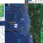
We just had an earthquake in the Gorda plate. The USGS magnitude is 5.1. This earthquake happened a few kilometers southwest of the 2014 M 6.8 earthquake. Based upon the orientation of the faults in the region, today’s earthquake may have occurred on the same fault as the 2014 earthquake (but it is really difficult to tell and just as likely did not).
The last earthquake report I prepared for a Gorda plate earthquake happened on 2016.09.25. Here is my report for that earthquake.

Here is the USGS website for this earthquake.

Below is my interpretive poster for this earthquake.

I plot the seismicity from the past month, with color representing depth and diameter representing magnitude (see legend).

  • I placed a moment tensor / focal mechanism legend on the poster. There is more material from the USGS web sites about moment tensors and focal mechanisms (the beach ball symbols). Both moment tensors and focal mechanisms are solutions to seismologic data that reveal two possible interpretations for fault orientation and sense of motion. One must use other information, like the regional tectonics, to interpret which of the two possibilities is more likely. Based upon the series of earthquakes and the mapped faults, I interpret this M 5.1 earthquake as a left-lateral strike-slip earthquake related to slip associated with the Gorda plate.
  • I also include the shaking intensity contours on the map. These use the Modified Mercalli Intensity Scale (MMI; see the legend on the map). This is based upon a computer model estimate of ground motions, different from the “Did You Feel It?” estimate of ground motions that is actually based on real observations. The MMI is a qualitative measure of shaking intensity. More on the MMI scale can be found here and here. This is based upon a computer model estimate of ground motions, different from the “Did You Feel It?” estimate of ground motions that is actually based on real observations.
  • I include the slab contours plotted (Hayes et al., 2012), which are contours that represent the depth to the subduction zone fault. These are mostly based upon seismicity. The depths of the earthquakes have considerable error and do not all occur along the subduction zone faults, so these slab contours are simply the best estimate for the location of the fault.

    I include some inset figures in the poster.

  • In the upper right corner is a map of the Cascadia subduction zone (CSZ) and regional tectonic plate boundary faults. This is modified from several sources (Chaytor et al., 2004; Nelson et al., 2004)
  • Below the CSZ map is an illustration modified from Plafker (1972). This figure shows how a subduction zone deforms between (interseismic) and during (coseismic) earthquakes. Today’s earthquake did not occur along the CSZ, so did not produce crustal deformation like this. However, it is useful to know this when studying the CSZ.
  • In the lower left corner is a figure from Rollins and Stein (2010). In their paper they discuss how static coulomb stress changes from earthquakes may impart (or remove) stress from adjacent crust/faults. I also present their figure where they present seismic observations for the 1983.08.24 M 5.5 earthquake (Rollins and Stein list M 6.3). I place a yellow star in the general location of today’s earthquake.
  • In the upper right corner is a map from Chaytor et al. (2004) that shows some details of the faulting in the region. More about this figure can be found below.


  • Here is a map of the Cascadia subduction zone, modified from Nelson et al. (2006). The Juan de Fuca and Gorda plates subduct norteastwardly beneath the North America plate at rates ranging from 29- to 45-mm/yr. Sites where evidence of past earthquakes (paleoseismology) are denoted by white dots. Where there is also evidence for past CSZ tsunami, there are black dots. These paleoseismology sites are labeled (e.g. Humboldt Bay). Some submarine paleoseismology core sites are also shown as grey dots. The two main spreading ridges are not labeled, but the northern one is the Juan de Fuca ridge (where oceanic crust is formed for the Juan de Fuca plate) and the southern one is the Gorda rise (where the oceanic crust is formed for the Gorda plate).

  • Here is a version of the CSZ cross section alone (Plafker, 1972). This shows two parts of the earthquake cycle: the interseismic part (between earthquakes) and the coseismic part (during earthquakes). Regions that experience uplift during the interseismic period tend to experience subsidence during the coseismic period.

  • Here is a map from Chaytor et al. (2004) that shows some details of the faulting in the region. The moment tensor (at the moment i write this) shows a north-south striking fault with a reverse or thrust faulting mechanism. While this region of faulting is dominated by strike slip faults (and most all prior earthquake moment tensors showed strike slip earthquakes), when strike slip faults bend, they can create compression (transpression) and extension (transtension). This transpressive or transtentional deformation may produce thrust/reverse earthquakes or normal fault earthquakes, respectively. The transverse ranges north of Los Angeles are an example of uplift/transpression due to the bend in the San Andreas fault in that region.

  • These are the models for tectonic deformation within the Gorda plate as presented by Jason Chaytor in 2004.
  • Mw = 5 Trinidad Chaytor

  • Here is a map from Rollins and Stein, showing their interpretations of different historic earthquakes in the region. This was published in response to the Januray 2010 Gorda plate earthquake. The faults are from Chaytor et al. (2004).

  • In this map below, I label a number of other significant earthquakes in this Mendocino triple junction region. Another historic right-lateral earthquake on the Mendocino fault system was in 1994. There was a series of earthquakes possibly along the easternmost section of the Mendocino fault system in late January 2015, here is my post about that earthquake series.

The Gorda and Juan de Fuca plates subduct beneath the North America plate to form the Cascadia subduction zone fault system. In 1992 there was a swarm of earthquakes with the magnitude Mw 7.2 Mainshock on 4/25. Initially this earthquake was interpreted to have been on the Cascadia subduction zone (CSZ). The moment tensor shows a compressional mechanism. However the two largest aftershocks on 4/26/1992 (Mw 6.5 and Mw 6.7), had strike-slip moment tensors. These two aftershocks align on what may be the eastern extension of the Mendocino fault.
There have been several series of intra-plate earthquakes in the Gorda plate. Two main shocks that I plot of this type of earthquake are the 1980 (Mw 7.2) and 2005 (Mw 7.2) earthquakes. I place orange lines approximately where the faults are that ruptured in 1980 and 2005. These are also plotted in the Rollins and Stein (2010) figure above. The Gorda plate is being deformed due to compression between the Pacific plate to the south and the Juan de Fuca plate to the north. Due to this north-south compression, the plate is deforming internally so that normal faults that formed at the spreading center (the Gorda Rise) are reactivated as left-lateral strike-slip faults. In 2014, there was another swarm of left-lateral earthquakes in the Gorda plate. I posted some material about the Gorda plate setting on this page.
There are three types of earthquakes, strike-slip, compressional (reverse or thrust, depending upon the dip of the fault), and extensional (normal). Here is are some animations of these three types of earthquake faults. Many of the earthquakes people are familiar with in the Mendocino triple junction region are either compressional or strike slip. The following three animations are from IRIS.
Strike Slip:

Compressional:

Extensional:


    References:

  • Atwater, B.F., Musumi-Rokkaku, S., Satake, K., Tsuju, Y., Eueda, K., and Yamaguchi, D.K., 2005. The Orphan Tsunami of 1700—Japanese Clues to a Parent Earthquake in North America, USGS Professional Paper 1707, USGS, Reston, VA, 144 pp.
  • Burgette, R. et al., 2009. Interseismic uplift rates for western Oregon and along-strike variation in locking on the Cascadia subduction zone in Journal of Geophysical Research, v. 114, B01408, doi:10.1029/2008JB005679
  • Chaytor, J.D., Goldfinger, C., Dziak, R.P., and Fox, C.G., 2004. Active deformation of the Gorda plate: Constraining deformation models with new geophysical data: Geology v. 32, p. 353-356
  • Goldfinger, C., Nelson, C.H., Morey, A., Johnson, J.E., Gutierrez-Pastor, J., Eriksson, A.T., Karabanov, E., Patton, J., Gràcia, E., Enkin, R., Dallimore, A., Dunhill, G., and Vallier, T., 2012. Turbidite Event History: Methods and Implications for Holocene Paleoseismicity of the Cascadia Subduction Zone, USGS Professional Paper # 1661F. U.S. Geological Survey, Reston, VA, 184 pp.
  • McCrory, P. A., Blair, J. L., Oppenheimer, D. H., and Walter, S. R., 2006. Depth to the Juan de Fuca slab beneath the Cascadia subduction margin; a 3-D model for sorting earthquakes U. S. Geological Survey
  • Nelson, A.R., Kelsey, H.M., and Witter, R.C., 2006. Great earthquakes of variable magnitude at the Cascadia subduction zone: Quaternary Research, doi:10.1016/j.yqres.2006.02.009, p. 354-365.
  • Plafker, G., 1972. Alaskan earthquake of 1964 and Chilean earthquake of 1960: Implications for arc tectonics in Journal of Geophysical Research, v. 77, p. 901-925.
  • Rollins, J.C., Stein, R.S., 2010. Coulomb Stress Interactions Among M ≥ 5.9 Earthquakes in the Gorda Deformation Zone and on the Mendocino Fault Zone, Cascadia Subduction Zone, and Northern San Andreas Fault. Journal of Geophysical Research 115, 19 pp.
  • USGS Quaternary Fault Database: http://earthquake.usgs.gov/hazards/qfaults/
  • Wang, K., Wells, R., Mazzotti, S., Hyndman, R. D., and Sagiya, T., 2003. A revised dislocation model of interseismic deformation of the Cascadia subduction zone Journal of Geophysical Research, B, Solid Earth and Planets v. 108, no. 1.

Earthquake Report: Turkey

We just had a good shaker in western Turkey. At the moment, there are over 400 reports of ground shaking to the USGS “Did you Feel It?” web page. The USGS PAGER report estimates that there may be some casualties (though a low number of them), but that the economic loss estimate is higher (35% chance of between 10 and 100 million USD).

This earthquake appears to have been along a normal fault named either the Bodum fault (NOA; Helenic Seismic Network) or the Ula-Oren fault (GreDASS; Greek Database of Seismogenic Sources). The inset map shows the faults and fault planes from the GreDASS database. A third name for this fault is the Gökova fault (Kurt et al., 1999).

Here is the USGS website for this earthquake.

There is lots of information on the European-Mediterranean Seismological Centre (EMSC) page here.

Below is my interpretive poster for this earthquake.

I plot the seismicity from the past month, with color representing depth and diameter representing magnitude (see legend). I also include USGS earthquake epicenters from 1917-2017 for magnitudes M ≥ 6.5. This is also the time and magnitude range of earthquakes in the inset map.

  • I placed a moment tensor / focal mechanism legend on the poster. There is more material from the USGS web sites about moment tensors and focal mechanisms (the beach ball symbols). Both moment tensors and focal mechanisms are solutions to seismologic data that reveal two possible interpretations for fault orientation and sense of motion. One must use other information, like the regional tectonics, to interpret which of the two possibilities is more likely. I plot moment tensors for the M 6.3 earthquake. Based upon the series of earthquakes and the mapped faults, I interpret this M 6.7 earthquake to be a normal fault (extensional) earthquake.
  • I also include the shaking intensity contours on the map. These use the Modified Mercalli Intensity Scale (MMI; see the legend on the map). This is based upon a computer model estimate of ground motions, different from the “Did You Feel It?” estimate of ground motions that is actually based on real observations. The MMI is a qualitative measure of shaking intensity. More on the MMI scale can be found here and here. This is based upon a computer model estimate of ground motions, different from the “Did You Feel It?” estimate of ground motions that is actually based on real observations.
  • I include the slab contours plotted from the (Database of Individual Seismogenic Sources (DISS), Version 3.2.0), which are contours that represent the depth to the subduction zone fault. These are mostly based upon seismicity. The depths of the earthquakes have considerable error and do not all occur along the subduction zone faults, so these slab contours are simply the best estimate for the location of the fault.

    I include some inset figures in the poster.

  • In the lower left corner I include a map of the regional tectonics (Dilek and Sandvol, 2009). I place a green star in the general location of today’s M 6.7 earthquake.
  • In the lower right corner is a figure from Jolivet et al. (2013) that shows focal mechanisms for earthquakes across the Aegean-Anatolian region. Earthquakes plotted in the region of today’s M 6.7 (the green star) are all normal (extensional) earthquakes (with one extensional oblique).
  • In the upper right corner is a tectonic map of western Eurasia and northern Africa (Dilek, 2006). Today’s earthquake lies near the cross section G-G (in yellow). I also show the general location of this cross-section on the main map.
  • Below this map is a figure showing a north-south cross section through this region (Dilek, 2006), G-G on the above map. This shows the subduction zone in the south, the transform fault (North Anatolian fault) in the north, and the Aegean Extensional Province in the center. Today’s earthquake is along the southern boundary of the core complex, which is in the center of this extensional province.
  • In the upper left corner is a larger scale map showing the same earthquakes as the main map. I also include the faults and fault planes from the GreDASS database. I also label the larger earthquakes in this region. Note the 2017 M 6.3 Lesbos earthquake in the north. Here is my earthquake report for that earthquake. Note the flare up of seismicity in the 1950s, possibly beginning in 1948.


  • Here is the same poster, but with USGS earthquake epicenters from 2007-2017 with magnitude M ≥ 4.5.

  • There was a small tsunami recorded at the Bodum tide gage. Here is the source.

  • Here is the tectonic map from Dilek and Sandvol (2009).

  • Tectonic map of the Aegean and eastern Mediterranean region showing the main plate boundaries, major suture zones, fault systems and tectonic units. Thick, white arrows depict the direction and magnitude (mm a21) of plate convergence; grey arrows mark the direction of extension (Miocene–Recent). Orange and purple delineate Eurasian and African plate affinities, respectively. Key to lettering: BF, Burdur fault; CACC, Central Anatolian Crystalline Complex; DKF, Datc¸a–Kale fault (part of the SW Anatolian Shear Zone); EAFZ, East Anatolian fault zone; EF, Ecemis fault; EKP, Erzurum–Kars Plateau; IASZ, Izmir–Ankara suture zone; IPS, Intra–Pontide suture zone; ITS, Inner–Tauride suture; KF, Kefalonia fault; KOTJ, Karliova triple junction; MM, Menderes massif; MS, Marmara Sea; MTR, Maras triple junction; NAFZ, North Anatolian fault zone; OF, Ovacik fault; PSF, Pampak–Sevan fault; TF, Tutak fault; TGF, Tuzgo¨lu¨ fault; TIP, Turkish–Iranian plateau (modified from Dilek 2006).

  • Below is a series of figures from Jolivet et al. (2013). These show various data sets and analyses for Greece and Turkey.
  • Upper Panel (A): This is a tectonic map showing the major faults and geologic terranes in the region. The fault possibly associated with today’s earthquake is labeled OU on the map, for the Ula-Oren fault.
  • Lower Panel (B): This shows historic seismicity for the region. Note the general correlation with the faults in the upper panel.

  • A: Tectonic map of the Aegean and Anatolian region showing the main active structures
    (black lines), the main sutures zones (thick violet or blue lines), the main thrusts in the Hellenides where they have not been reworked by later extension (thin blue lines), the North Cycladic Detachment (NCDS, in red) and its extension in the Simav Detachment (SD), the main metamorphic units and their contacts; AlW: Almyropotamos window; BD: Bey Daglari; CB: Cycladic Basement; CBBT: Cycladic Basement basal thrust; CBS: Cycladic Blueschists; CHSZ: Central Hellenic Shear Zone; CR: Corinth Rift; CRMC: Central Rhodope Metamorphic Complex; GT: Gavrovo–Tripolitza Nappe; KD: Kazdag dome; KeD: Kerdylion Detachment; KKD: Kesebir–Kardamos dome; KT: Kephalonia Transform Fault; LN: Lycian Nappes; LNBT: Lycian Nappes Basal Thrust; MCC: Metamorphic Core Complex; MG: Menderes Grabens; NAT: North Aegean Trough; NCDS: North Cycladic Detachment System; NSZ: Nestos Shear Zone; OlW: Olympos Window; OsW: Ossa Window; OSZ: Ören Shear Zone; Pel.: Peloponnese; ÖU: Ören Unit; PQN: Phyllite–Quartzite Nappe; SiD: Simav Detachment; SRCC: South Rhodope Core Complex; StD: Strymon Detachment; WCDS: West Cycladic Detachment System; ZD: Zaroukla Detachment. B: Seismicity. Earthquakes are taken from the USGS-NEIC database. Colour of symbols gives the depth (blue for shallow depths) and size gives the magnitude (from 4.5 to 7.6).

  • Upper Panel (C): These red arrows are Global Positioning System (GPS) velocity vectors. The velocity scale vector is in the lower left corner. The main geodetic (study of plate motions and deformation of the earth) signal here is the westward motion of the North Anatolian fault system as it rotates southward as it traverses Greece. The motion trends almost south near the island of Crete, which is perpendicular to the subduction zone.
  • Lower Panel (D): This map shows the region of mid-Cenozoic (Oligo-Miocene) extension (shaded orange). It just happens that there is still extension going on in parts of this prehistoric extension.

  • C: GPS velocity field with a fixed Eurasia after Reilinger et al. (2010) D: the domain affected by distributed post-orogenic extension in the Oligocene and the Miocene and the stretching lineations in the exhumed metamorphic complexes.

  • Upper Panel (E): This map shows where the downgoing slab may be located (in blue), along with the volcanic centers associated with the subduction zone in the past.
  • Lower Panel (F): This map shows the orientation of how seismic waves orient themselves differently in different places (anisotropy). We think seismic waves travel in ways that reflects how tectonic strain is stored in the earth. The blue lines show the direction of extension in the asthenosphere, green lines in the lithospheric mantle, and red lines for the crust.

  • E: The thick blue lines illustrate the schematized position of the slab at ~150 km according to the tomographic model of Piromallo and Morelli (2003), and show the disruption of the slab at three positions and possible ages of these tears discussed in the text. Velocity anomalies are displayed in percentages with respect to the reference model sp6 (Morelli and Dziewonski, 1993). Coloured symbols represent the volcanic centres between 0 and 3 Ma after Pe-Piper and Piper (2006). F: Seismic anisotropy obtained from SKS waves (blue bars, Paul et al., 2010) and Rayleigh waves (green and orange bars, Endrun et al., 2011). See also Sandvol et al. (2003). Blue lines show the direction of stretching in the asthenosphere, green bars represent the stretching in the lithospheric mantle and orange bars in the lower crust.

  • Upper Panel (G): This is the map showing focal mechanisms in the poster above. Note the strike slip earthquakes associated with the North Anatolian fault and the thrust/reverse mechanisms associated with the thrust faults.

  • G: Focal mechanisms of earthquakes over the Aegean Anatolian region.

  • Here is a figure showing a north-south cross section through this region, from ~95 million years ago until about 2 million years ago (Dilek and Sandvol, 2009). This figure shows how the regional tectonics have developed over time, with the modern subduction zone in the south, the North Anatolian transform fault in the north, and an extensional metamorphic core complex in the center (“Core Complex” on cross section). Today’s earthquake is along the southern boundary of this core complex.

  • Late Mesozoic–Cenozoic geodynamic evolution of the western Anatolian orogenic belt as a result of collisional and extensional processes in the upper plate of north-dipping subduction zone(s) within the Tethyan realm.

  • This is a great figure showing another interpretation to explain the extension in this region (slab rollback and mantle flow) from Brun and Sokoutis (2012).

  • Mantle flow pattern at Aegean scale powered by slab rollback in rotation around vertical axis located at Scutary-Pec (Albania). A: Map view of flow lines above (red) and below (blue) slab. B: Three-dimensional sketch showing how slab tear may accommodate slab rotation. Mantle fl ow above and below slab in red and blue, respectively. Yellow arrows show crustal stretching.

  • Finally, here is a map showing tectonic domains (Taymaz et al., 2007).

  • Schematic map of the principal tectonic settings in the Eastern Mediterranean. Hatching shows areas of coherent motion and zones of distributed deformation. Large arrows designate generalized regional motion (in mm a21) and errors (recompiled after McClusky et al. (2000, 2003). NAF, North Anatolian Fault; EAF, East Anatolian Fault; DSF, Dead Sea Fault; NEAF, North East Anatolian Fault; EPF, Ezinepazarı Fault; CTF, Cephalonia Transform Fault; PTF, Paphos Transform Fault.

References

  • Basili R., G. Valensise, P. Vannoli, P. Burrato, U. Fracassi, S. Mariano, M.M. Tiberti, E. Boschi (2008), The Database of Individual Seismogenic Sources (DISS), version 3: summarizing 20 years of research on Italy’s earthquake geology, Tectonophysics, doi:10.1016/j.tecto.2007.04.014
  • Brun, J.-P., Sokoutis, D., 2012. 45 m.y. of Aegean crust and mantle flow driven by trench retreat. Geol. Soc. Am., v. 38, p. 815–818.
  • Caputo, R., Chatzipetros, A., Pavlides, S., and Sboras, S., 2012. The Greek Database of Seismogenic Sources (GreDaSS): state-of-the-art for northern Greece in Annals of Geophysics, v. 55, no. 5, doi: 10.4401/ag-5168
  • Dilek, Y., 2006. Collision tectonics of the Mediterranean region: Causes and consequences in Dilek, Y., and Pavlides, S., eds., Postcollisional tectonics and magmatism in the Mediterranean region and Asia: Geological Society of America Special Paper 409, p. 1–13
  • Dilek, Y. and Sandvol, E., 2006. Collision tectonics of the Mediterranean region: Causes and consequences in Dilek, Y., and Pavlides, S., eds., Postcollisional tectonics and magmatism in the Mediterranean region and Asia: Geological Society of America Special Paper 409, p. 1–13
  • DISS Working Group (2015). Database of Individual Seismogenic Sources (DISS), Version 3.2.0: A compilation of potential sources for earthquakes larger than M 5.5 in Italy and surrounding areas. http://diss.rm.ingv.it/diss/, Istituto Nazionale di Geofisica e Vulcanologia; DOI:10.6092/INGV.IT-DISS3.2.0.
  • Ersoy, E.Y., Cemen, I., Helvaci, C., and Billor, Z., 2014. Tectono-stratigraphy of the Neogene basins in Western Turkey: Implications for tectonic evolution of the Aegean Extended Region in Tectonophysics v. 635, p. 33-58.
  • Jolivet, L., et al., 2013. Aegean tectonics: Strain localisation, slab tearing and trench retreat in Tectonophysics, v. 597-598, p. 1-33
  • Kokkalas, S., et al., 2006. Postcollisional contractional and extensional deformation in the Aegean region in GSA Special Papers, v. 409, p. 97-123.
  • Kurt, H., Demirbag, E., and Kuscu, I., 1999. Investigation of the submarine active tectonism in the Gulf of Gokova, southwest Anatolia–southeast Aegean Sea, by multi-channel seismic reflection data in Tectonophysics, v. 305, p. 477-496
  • Papazachos, B.C., Papadimitrious, E.E., Kiratzi, A.A., Papazachos, C.B., and Louvari, E.k., 1998. Fault Plane Solutions in the Aegean Sea and the Surrounding Area and their Tectonic Implication, in Bollettino Di Geofisica Terorica Ed Applicata, v. 39, no. 3, p. 199-218.
  • Taymaz, T., Yilmaz, Y., and Dilek, Y., 2007. The geodynamics of the Aegean and Anatolia: introduction in Geological Society Special Publications, v. 291, p. 1-16.
  • Wouldloper, 2009. Tectonic map of southern Europe and the Middle East, showing tectonic structures of the western Alpide mountain belt. Only Alpine (tertiary) structures are shown.

Earthquake Report: Bering fracture zone: UPDATE #1

Well, based upon a comment on twitter, I thought it prudent to review the seismicity of this region at the westernmost part of the western Aleutian Islands. For many years I considered this region part of the subduction zone that forms the Aleutian Trench. In the past couple of years, there have been a number of earthquakes that reveal this to not be the case. Rather, the Pacific-North America plate boundary in this region is in the form of a shear zone, distributed across several reactivated fracture zones. I noticed a plot from Jascha Polet and found another article that evaluates this plate boundary (Davaille and Lees, 2004).

Here is my initial #EarthquakeReport on this M 7.7 strike-slip earthquake.

Here is a report from the University of Alaska Fairbanks, Alaska Earthquake Center.

Below is my interpretive poster for this earthquake.

  • I placed a moment tensor / focal mechanism legend on the poster. There is more material from the USGS web sites about moment tensors and focal mechanisms (the beach ball symbols). Both moment tensors and focal mechanisms are solutions to seismologic data that reveal two possible interpretations for fault orientation and sense of motion. One must use other information, like the regional tectonics, to interpret which of the two possibilities is more likely. I plot moment tensors for the M 7.7 earthquake. Based upon the series of earthquakes and the mapped faults, I interpret this M 7.7 earthquake as a right-lateral strike-slip earthquake related to slip associated with the Bering fracture zone.
  • I also include the shaking intensity contours on the map. These use the Modified Mercalli Intensity Scale (MMI; see the legend on the map). This is based upon a computer model estimate of ground motions, different from the “Did You Feel It?” estimate of ground motions that is actually based on real observations. The MMI is a qualitative measure of shaking intensity. More on the MMI scale can be found here and here. This is based upon a computer model estimate of ground motions, different from the “Did You Feel It?” estimate of ground motions that is actually based on real observations.
  • I include the slab contours plotted (Hayes et al., 2012), which are contours that represent the depth to the subduction zone fault. These are mostly based upon seismicity. The depths of the earthquakes have considerable error and do not all occur along the subduction zone faults, so these slab contours are simply the best estimate for the location of the fault.
  • I plot the seismicity from the past month, with color representing depth and diameter representing magnitude (see legend). I also include USGS earthquake epicenters from 1917-2017 for magnitudes M ≥ 5.0. The depths for these earthquakes is represented by color. This is quite revealing when considering whether subduction is occurring in this part of the plate boundary. Note how earthquakes east of Attu Island have hypocentral depths (3-dimensional location of the earthquake focus) that extend to over 150 km. These represent earthquakes in the downgoing Pacific plate. We also observe earthquakes even deeper along the Kamchatka Trench on the west. Also note that the slab contours (Hayes et al., 2012) have decreasing maximum depths from east to west between Bowers Ridge and Attu Island. The same is true for the subduction zone beneath Kamchatka, though the cut-off of these depth contours is more abrupt (due to the tear in the Pacific plate, which marks the edge of the subduction zone beneath Kamchatka). Finally, note how the earthquake depths in the region between Attu Island and Kamchatka are largely less than 33 km.

    I include some inset figures in the poster.

  • In the upper left corner I include a regional tectonic map showing Kamchatka and the westernmost tip of the westernmost Aleutian Islands (Davaille and Lees, 2004).
  • In the lower right corner I show a schematic illustration that depicts how the subduction transitions to strike-slip in the region of the Attu Island (Davaille and Lees, 2004).
  • To the right is a large scale map of this region showing the complicated intersection of strike slip and compressional tectonics as the tip of the Aleutians intersects with Kamchatka (Gaedicke et al., 2000).
  • In the upper right corner is a figure showing seismicity in this region (Davaille and Lees, 2004). There is a map (with earthquakes plotted vs. depth in color) and several cross sections (one parallel to the Kamchatka trench and two normal/perpendicular to the trench). Note how the depths for the earthquakes shallow to the north of the Meiji Seamount, and particularly shallower to the north of the Stellar fault (a.k.a. Bering Kresla Shear zone) and the Bering fault (a.k.a. Bering fracture zone).


  • Here is my original #EarthquakeReport Interpretive Poster and report.

  • Here is the seismicity plot from Davaille and Lees (2000). They suspect that the tear in the Pacific plate is related to the interaction of a mantle plume hotspot and the oceanic lithosphere as it is formed near this hotspot. I include their figure caption below in blockquote.

  • Seismicity in Kamchatka. (a) Mapview showing earthquakes plotted with colors corresponding to depth. Projections of the Bering and Steller faults onto Kamchatka are presented for clarity and reference. (b–d) Vertical cross-sections of seismicity in Kamchatka. Magenta circles are from the Gorbatov et al. [3] catalog and yellow events are from the Engdahl et al. [52] catalog. The projection of the subducting Meiji seamounts is shaded gray.

  • Here is a plot from Jascha Polet, seismologist at Cal Poly Pomona. These data are consistent with the Davaille and Lees (2000) plot, showing shallow seismicity in this region of the plate boundary.

  • Here is the low-angle oblique map from Portnyagin and Manea (2008). This was in my original report, but is a great visualization for this interpretation of the Pacific plate tear (the edge of subduction in Kamchatka). While this is not evidence for the lack of subduction in the region of the Bering Kresla Shear zone, it does suggest that there is no active subduction beneath Kamchatka to the north. If this is the case (and I have no reason to think that it is not the case), there is little evidence for subduction west of Attu Island and east of Kamchatka. I include the figure caption as a blockquote below.

  • Kamchatka subduction zone. A: Major geologic structures at the Kamchatka–Aleutian Arc junction. Thin dashed lines show isodepths to subducting Pacific plate (Gorbatov et al., 1997). Inset illustrates major volcanic zones in Kamchatka: EVB—Eastern Volcanic Belt; CKD—Central Kamchatka Depression (rift-like tectonic structure, which accommodates the northern end of EVB); SR—Sredinny Range. Distribution of Quaternary volcanic rocks in EVB and SR is shown in orange and green, respectively. Small dots are active vol canoes. Large circles denote CKD volcanoes: T—Tolbachik; K l — K l y u c h e v s k o y ; Z—Zarechny; Kh—Kharchinsky; Sh—Shiveluch; Shs—Shisheisky Complex; N—Nachikinsky. Location of profiles shown in Figures 2 and 3 is indicated. B: Three dimensional visualization of the Kamchatka subduction zone from the north. Surface relief is shown as semi-transparent layer. Labeled dashed lines and color (blue to red) gradation of subducting plate denote depths to the plate from the earth surface (in km). Bold arrow shows direction of Pacific Plate movement.

  • Here is another great visualization of the subducting slabs in this region, prepared by Lees et al. (2007). This figure shows isosurfaces (surfaces of equal value of some parameter, like seismic velocity, or Vp:Vs ratios; Vp = P-Wave velocity, Vs = S-Wave velocity). These isosurfaces were created using seismic tomography, which is basically just like a CT scan of the earth. CT stands for “computed tomography” of X-Rays. The mathematical solutions used in these methods are the same, even though the source of the data are different (X-Rays vs. seismic waves). Coastlines are in grey outline. Kamchatka is labelled M. The lower panel may be easier to look at first because north is up. Basically, blue is old and cold and red is young and hot. So, the downgoing Pacific plate is in blue and the surrounding mantle is in red. Note how the blue blobs end in the area of interest.

  • Tomographic image of the Kamchatka Subduction zone rendered in three-dimensions. The cut-off perturbation level is 3% with blue regions being high velocity and red lower velocity perturbations. The slab is a clear high velocity zone approximately 100 km thick plunging into the upper mantle at an angle of ~50. The green plane represents the top of the subduction zone seismicity, contoured and rendered along with the tomographic images. Gold cones are active volcanoes along the Kamchatka arc and white squares are stations included for reference to the map in Figure 1. The bars represent length scales of 100 km. Points of interest discussed in the text are marked with letters (I–M).

  • Finally of note (unrelated to the previous discussion) is that this M 7.7 had a really long duration (Dr. Polet pointed this out in a tweet). This plot is from IPGP here. The source time function represents how much energy is released over time. Time is on the horizontal axis.

    References:

  • Bassett and Watts, 2015. Gravity anomalies, crustal structure, and seismicity at subduction zones: 1. Seafloor roughness and subducting relief in Geochemistry, Geophysics, Geosystems, v. 16, doi:10.1002/2014GC005684.
  • Davaille, A. and Lees, J.M., 2004. Thermal modeling of subducted plates: tear and hotspot at the Kamchatka corner in EPSL, v. 226, p. 293-304.
  • Gaedicke, C., Baranov, B., Seliverstov, N., Alexeiev, D., Tsukanov, N., Freitag, R., 2000. Structure of an active arc-continent collision area: the Aleutian-Kamchatka junction. Tectonophysics 325, 63–85
  • Hayes, G. P., D. J. Wald, and R. L. Johnson (2012), Slab1.0: A three-dimensional model of global subduction zone geometries, J. Geophys. Res., 117, B01302, doi:10.1029/2011JB008524.
  • Ikuta, R., Mitsui, Y., Kurokawa, Y., and Ando, M., 2015. Evaluation of strain accumulation in global subduction zones from seismicity data in Earth, Planets and Space, v. 67, DOI 10.1186/s40623-015-0361-5
  • Konstantnovskaia, 2001. Arc-continent collision and subduction reversal in the Cenozoic evolution of the Northwest Pacific: an example from Kamchatka (NE Russia) in Tectonophysics, v. 333, p. 75-94.
  • Koulakov, I.Y., Dobretsov, N.L., Bushenkova, N.A., and Yakovlev, A.V., 2011. Slab shape in subduction zones beneath the Kurile–Kamchatka and Aleutian arcs based on regional tomography results in Russian Geology and Geophysics, v. 52, p. 650-667.
  • Krutikov, L., et al., 2008. Active Tectonics and Seismic Potential of Alaska, Geophysical Monograph Series 179, doi:10.1029/179GM07
  • Lees, J.M., VanDecar, J., Gordeev, E., Ozerov, A., Brandon, M., Park, J., and Levvin, V, 2007. Three Dimensional Images of the Kamchatka-Pacific Plate Cusp in Volcanism and Subduction: The Kamchatka Region Geophysical Monograph Series 172, DOI: 10.1029/172GM06
  • Portnyagin, M. and Manea, V.C., 2008. Mantle temperature control on composition of arc magmas along the Central Kamchatka Depression in Geology, v. 36, no. 7, p. 519-522.
  • Rhea, S., Tarr, A.C., Hayes, G., Villaseñor, A., Furlong, K.P., and Benz, H.M., 2010. Seismicity of the Earth 1900-2007, Kuril-Kamchatka arc and vicinity: U.S. Geological Survey Open-File Report 2010-1083-C, 1 map sheet, scale 1:5,000,000.

Earthquake Report: Western Aleutians

We just had an earthquake along the western Aleutian Islands, very close to the international date line. In this region places often have more than two names, depending upon who drew the map.

The majority of the Aleutian Islands are volcanic arc islands formed as a result of the subduction of the Pacific plate beneath the North America plate. To the west, there is another subduction zone along the Kuril and Kamchatka volcanic arcs. These subduction zones form deep sea trenches (the deepest parts of the ocean are in subduction zone trenches). Between these 2 subduction zones is another linear trough, but this does not denote the location of a subduction zone. The plate boundary between the Kamchatka and Aleutian trenches is the Bering Kresla shear zone (BKSZ).

The oceanic basin, Komandorsky Basin, to the north of the BKSZ has been mapped with northwest trending fracture zones, most of which are fossil or inactive. However, due to the oblique convergence west of Bowers Ridge, some of these fossil fracture zones are being reactivated. Based upon offsets in magnetic anomalies in the oceanic crust forming the basement of Komandorsky Basin, these fracture zones show left-lateral offsets. However, the active strike-slip faults (and BKSZ) are right lateral. This is a great example of strike-slip faults reactivating as strike-slip faults.

The mainshock was preceded earlier this day with several foreshocks and occurred very close to a M 6.3 earthquake from 9 months ago (2016.09.05). In addition, there was seismic activity to the east about 6 weeks ago (2017.06.02 M 6.8).

Some place a tear in the downgoing Pacific plate (beneath Kamchatka) in the position of the Bering Kresla Shear zone. This marks the end of the modern Kamchatka subduction zone. However, there was a subduction zone further to the west of the active arc, which extended further to the north and possibly involved subduction of the oceanic crust forming the Komandorsky Basin. The combination of offsets along the right-lateral strike-slip faults to the north of the BKSZ, along with the convergence along the Kamchatka Trench, there is a fold and thrust belt (a zone of compressional tectonics). There was an M 6.6 earthquake earlier this year (2017.03.29), which is somewhat related to this fold and thrust belt.

Finally, of note, is the M 8.3 deep extensional earthquake in the downgoing Pacific plate crust (2013.05.24).

There was a tsunami recorded at the tide gage on Shemya Island, with an observed maximum wave height of 0.3 ft! This is interesting given the strike slip earthquake.

  • Here are the USGS website for today’s earthquakes.
  • 2017-07-17 11:05 M 6.2
  • 2017-07-17 11:23 M 5.1
  • 2017-07-17 23:34 M 7.7
  • Here are my #EarthquakeReport pages for some of these related earthquakes.
  • 2016.09.05 M 6.3
  • 2017.03.29 M 6.6
  • 2017.06.02 M 6.8

Below is my interpretive poster for this earthquake.

I plot the seismicity from the past month, with color representing depth and diameter representing magnitude (see legend). I also include USGS earthquake epicenters from 2007-2017 for magnitudes M ≥ 6.0.

  • I placed a moment tensor / focal mechanism legend on the poster. There is more material from the USGS web sites about moment tensors and focal mechanisms (the beach ball symbols). Both moment tensors and focal mechanisms are solutions to seismologic data that reveal two possible interpretations for fault orientation and sense of motion. One must use other information, like the regional tectonics, to interpret which of the two possibilities is more likely. I plot moment tensors for the M 7.7 earthquake, as well as for the 2013, 2016, and 2017 earthquakes mentioned above. I also include moment tensors for earthquakes in 1999 and 2001 because these are also interesting earthquakes that I had not noticed before. It appears that perhaps the 1999 strike-slip earthquake led to an increased stress on the subduction zone, which slipped in 2001. Based upon the series of earthquakes and the mapped faults, I interpret this M 7.7 earthquake as a right-lateral strike-slip earthquake related to slip associated with the Bering fracture zone.
  • I also include the shaking intensity contours on the map. These use the Modified Mercalli Intensity Scale (MMI; see the legend on the map). This is based upon a computer model estimate of ground motions, different from the “Did You Feel It?” estimate of ground motions that is actually based on real observations. The MMI is a qualitative measure of shaking intensity. More on the MMI scale can be found here and here. This is based upon a computer model estimate of ground motions, different from the “Did You Feel It?” estimate of ground motions that is actually based on real observations.
  • I include the slab contours plotted (Hayes et al., 2012), which are contours that represent the depth to the subduction zone fault. These are mostly based upon seismicity. The depths of the earthquakes have considerable error and do not all occur along the subduction zone faults, so these slab contours are simply the best estimate for the location of the fault.

    I include some inset figures in the poster.

  • In the upper left corner I include a regional tectonic map showing Kamchatka and the westernmost tip of the westernmost Aleutian Islands (Bindeman et a., 2002). Today’s M 7.7 earthquake is just off the map to the east.
  • To the right of the Bindeman map is a map that shows a larger scale view of the faults in this region (Gaedicke et al., 2000). I include an orange star designating the rough location of today’s M 7.7 earthquake.
  • In the lower left corner are the earthquake intensity regression plots for the M 6.2 and M 7.7 earthquakes. These are plots based upon Attenuation Relation equations (formerly called Ground Motion Prediction Equations, GMPEs). Using seismic data from thousands of earthquakes with a range of magnitudes, distances, fault types, etc., people have developed empirical relations between each of these parameters. These plots are based upon these empirical relations and show how earthquake intensity (how strong it shakes) diminishes with distance.
  • In the upper right corner is a series of tectonic maps showing one interpretation of how the plates have moved relative to each other through time (Konstantinovskaia, 2001). The time spans 65, 55, and 37 millions of years into the present. Begin by looking at the present configuration and move backwards in time. These maps show an interesting story (that appears consistent with other published data).


  • Here are several figures from Gaedicke et al. (2000) showing their tectonic reconstructions. I include their figure captions below in blockquote. The first map shows the general tectonic setting as in the poster above.

  • Map of the Aleutian–Bering region and location of the study area (rectangle). Lines with barbs indicate subduction zones: (1) Kamchatka Trench and (2) Aleutian Trench; lines with sense of displacement mark fracture zones (FZs): (3) Steller, (4) Pikezh and (5) Bering FZs. Single arrows show relative direction of convergence of the Pacific (P) and North American (NA) plates. Bathymetric contours are in meters.

  • This figure shows the complicated intersection of the BKSZ and the Kuril-Kamchatka Trench (a subduction zone).

  • The main tectonic features of the Kamchatka–Aleutian junction area modified from Seliverstov (1983), Seliverstov et al. (1988) and Baranov et al. (1991). The eastern side of the Central Kamchatka depression is bounded by normal faults. Contour interval is 1000 m. Lines A and B indicate the locations of profiles shown in Fig. 3; the rectangle marks the location of the area shown in Fig. 4.

  • This figure shows a medium scale view of the faults here, along with the major historic earthquakes. In this figure the BKSZ is labeled the Aleutian fracture zone (AFZ).

  • Rupture zones of the major earthquakes in the Kamchatka–Aleutian junction area [according to Vikulin (1997)]. Earthquakes with a magnitude of Mw>7 are shown.

  • Here are several figures from Konstantnovskaia et al. (2001) showing their tectonic reconstructions. I include their figure captions below in blockquote. The first figure is the one included in the poster above.

  • Geodynamic setting of Kamchatka in framework of the Northwest Pacific. Modified after Nokleberg et al. (1994) and Kharakhinov (1996)). Simplified cross-section line I-I’ is shown in Fig. 2. The inset shows location of Sredinny and Eastern Ranges. [More figure caption text in the publication].

  • Here are 4 panels that show the details of their reconstructions. Panels shown are for 65 Ma, 55 Ma, 37 Ma, and Present.


  • The Cenozoic evolution in the Northwest Pacific. Plate kinematics is shown in hotspot reference frame after (Engebretson et al., 1985). Keys distinguish zones of active volcanism (thick black lines), inactive volcanic belts (thick gray lines), deformed arc terranes (hatched pattern), subduction zones: active (black triangles), inactive *(empty triangles). In letters: sa = Sikhote-aline, bs = Bering shelf belts; SH = Shirshov Ridge; V = Vitus arch; KA = Kuril; RA = Ryukyu’ LA = Luzon; IBMA = Izu-Bonin-Mariana arcs; WPB = Western Philippine, BB = Bowers basins.

  • Here is the low-angle oblique map from Portnyagin and Manea (2008). I include the figure caption as a blockquote below.

  • Kamchatka subduction zone. A: Major geologic structures at the Kamchatka–Aleutian Arc junction. Thin dashed lines show isodepths to subducting Pacific plate (Gorbatov et al., 1997). Inset illustrates major volcanic zones in Kamchatka: EVB—Eastern Volcanic Belt; CKD—Central Kamchatka Depression (rift-like tectonic structure, which accommodates the northern end of EVB); SR—Sredinny Range. Distribution of Quaternary volcanic rocks in EVB and SR is shown in orange and green, respectively. Small dots are active vol canoes. Large circles denote CKD volcanoes: T—Tolbachik; K l — K l y u c h e v s k o y ; Z—Zarechny; Kh—Kharchinsky; Sh—Shiveluch; Shs—Shisheisky Complex; N—Nachikinsky. Location of profiles shown in Figures 2 and 3 is indicated. B: Three dimensional visualization of the Kamchatka subduction zone from the north. Surface relief is shown as semi-transparent layer. Labeled dashed lines and color (blue to red) gradation of subducting plate denote depths to the plate from the earth surface (in km). Bold arrow shows direction of Pacific Plate movement.