Earthquake Report: Sulawesi, Indonesia

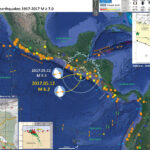
There was a series of earthquakes in Sulawesi, Indonesia earlier today, with a mainshock having a magnitude of M 6.8. This series of earthquakes is interesting as it does not occur on the main plate boundary fault, but on upper plate faults in the region. There is a major left-lateral strike-slip fault system to the west of these earthquakes (the Palu-Koro fault).
Part of this being interesting is that the orientation of the earthquake is oblique to some estimates of the orientation of extension in this region. The M 6.8 earthquake shows an extensional earthquake with extension oriented ~north-south. Some estimate extension in the upper plate to be northeast-southwest (Bellier et al., 2006), while others estimate extension in the upper plate to be oriented parallel to the M 6.8 earthquake (e.g. Walpersdorf et al., 1998). Spencer (2010) also documented normal faults in the upper plate that may also be correctly oriented for this M 6.8 earthquake. However, looking at the SRTM topographic data using the GeoMapApp, there is a structural grain that appears oriented to the extension estimated by Bellier et al., 2006.

  • Here are the USGS earthquake websites for this sequence.
  • 2017.05.29 14:35 M 6.8
  • 2017.05.29 14:53 M 4.7
  • 2017.05.29 15:04 M 5.1
  • 2017.05.29 15:18 M 5.1

Below is my interpretive poster for this earthquake.

I plot the seismicity from the past month, with color representing depth and diameter representing magnitude (see legend). I also include seismicity from 1917-2017 for earthquakes with magnitudes M ≥ 7.5. Here is the USGS derived Google Earth kml file I used to create this map. I show the fault plane solutions for one of these earthquakes (1996 M 7.9). The 1996 M 7.9 earthquake is oriented with the subduction fault on the north side of Sulawesi. Interestingly, there is no seismicity M ≥ 7.5 along the strike-slip systems here.

  • I placed a moment tensor / focal mechanism legend on the poster. There is more material from the USGS web sites about moment tensors and focal mechanisms (the beach ball symbols). Both moment tensors and focal mechanisms are solutions to seismologic data that reveal two possible interpretations for fault orientation and sense of motion. One must use other information, like the regional tectonics, to interpret which of the two possibilities is more likely
  • I also include the shaking intensity contours on the map. These use the Modified Mercalli Intensity Scale (MMI; see the legend on the map). This is based upon a computer model estimate of ground motions, different from the “Did You Feel It?” estimate of ground motions that is actually based on real observations. The MMI is a qualitative measure of shaking intensity. More on the MMI scale can be found here and here. This is based upon a computer model estimate of ground motions, different from the “Did You Feel It?” estimate of ground motions that is actually based on real observations.
  • I did not include the slab contours plotted (Hayes et al., 2012), which are contours that represent the depth to the subduction zone fault. These are mostly based upon seismicity. The depths of the earthquakes have considerable error and do not all occur along the subduction zone faults, so these slab contours are simply the best estimate for the location of the fault. The hypocentral depth plots this close to the location of the fault as mapped by Hayes et al. (2012).

    I include some inset figures in the poster.

  • In the lower left corner is a general tectonic map for this part of the world (Zahirovic et al., 2014). I placed a green star in the location of this M 6.8 earthquake.
  • In the lower right corner is a low-angle oblique view of the plate boundaries in the northern part of this region (Hall, 2011). The upper part of the diagram shows the opposing vergent subduction zones along that strike north-south along the Molucca Strait (Halmahera, Philippines). The lower panel shows the downgoing Australia plate along the Timor Trench and Seram Trench.. I placed a green star in the location of this M 6.8 earthquake.
  • In the upper right corner I include an inset of a seismic hazard map for this region of Indonesia. This map is from the Indonesian National Agency for Disaster Management (2011). Note the high seismic hazard associated with the Palu-Koro and Matano faults.
  • In the upper right corner I include a tectonic map showing the major fault systems and generalized plate motions (Bellier et al., 2006). Note the northeast-southwest orientation of extension in the Central Sulawesi block. I present another figure from this publication below.
  • To the right of this Bellier et al. (2006) map is another figure from that same publication. This is more generalized and shows the orientation of the faults in this region.


  • Here is the tectonic map from Bellier et al., 2006. I include their caption below in blockquote.


  • Regional geodynamic sketch that presents the present day deformation model of Sulawesi area (after Beaudouin et al., 2003) and four main deformation systems around the Central Sulawesi block, highlighting the tectonic complexity of Sulawesi. Approximate location of the Central Sulawesi block rotation pole (P) [compatible with both GPS measurements (Walpersdorf et al., 1998a) and earthquake moment tensor analyses (Beaudouin et al., 2003)], as well as the major active structures are reported. Central Sulawesi Fault System (CSFS) is formed by the Palu–Koro and Matano faults. Arrows correspond to the compression and/or extension directions deduced from both inversion and moment tensor analyses of the focal mechanisms; arrow size being proportional to the deformation rate (e.g., Beaudouin et al., 2003).We also represent the focal mechanism provided by the Harvard CMT database [CMT data base, 2005] for the recent large earthquake (Mw=6.2; 2005/1/23; lat.=0.928S; long.=120.108E). The box indicates the approximate location of the Fig. 6 that corresponds to the geological map of the Palu basin region. The bottom inset shows the SE Asia and Sulawesi geodynamic frame where arrows represent the approximate Indo-Australian and Philippines plate motions relative to Eurasia.

  • Here is the larger scale map showing the fault configuration in this region (Bellier et al., 2006)


  • Sketch map of the Cenozoic Central Sulawesi fault system. ML represents the Matano Lake, and Leboni RFZ, the Leboni releasing fault zone that connects the Palu–Koro and Matano Faults. Triangles indicate faults with reverse component (triangles on the upthrown block). On this map are reported the fault kinematic measurement sites (geographic coordinates in Table 3).

  • The extension shown in the Bellier et al. (2006) map above is largely the result of analyses conducted by and presented in Beaudouin et al. (2003). Here I present their figure where they summarize their results of block modeling using historic seismicity to drive the strain in this region. It is possible that the century of seismicity data is insufficient to account for the strain here. This may explain why the orientation of the M 6.8 earthquake is not oriented like suggested in this map below.


  • Here is a figure from Walpersdorf et al. (1998) that shows regional plate motions and the tectonic faults in the region. Note that the extension is oriented parallel to the M 6.8 extension. These data are based upon their analyses of GPS geodetic data. So, given the orientation of the M 6.8 earthquake and these data, I suspect this is the correct orientation of extension. Though, this is not consistent with the topographic data I present below.


  • Distribution of the calk alkalic potassic (CAK) volcanism in Sulawesi. In the west arm this volcanism is restricted to the central part of the arm, while east of the Palu–Koro fault zone CAK volcanism is distributed across a NW–SE 200 km wide belt extending from north Sulawesi to the Una-Una Island. The two synthetic cross sections illustrate the contrasting distribution of this volcanism on both sides of the Palu–Koro fault zone. Extension of the Sula-Buton=north Sulawesi arc is speculative. The double arrow illustrates extension in the Gulf of Gorontalo. Dashed lines in cross sections indicate the presence at depth of the remnant subducted Tethys oceanic crust.

  • This is smaller scale tectonic map of the region (Zahirovic et al., 2014).

  • Regional tectonic setting with plate boundaries (MORs/transforms = black, subduction zones = teethed red) from Bird (2003) and ophiolite belts representing sutures modified from Hutchison (1975) and Baldwin et al. (2012). West Sulawesi basalts are from Polvé et al. (1997), fracture zones are from Matthews et al. (2011) and basin outlines are from Hearn et al. (2003). ANI – Andaman and Nicobar Islands, BD– Billiton Depression, Ba – Bangka Island, BI – Belitung (Billiton) Island, BiS – Bismarck Sea, BP – Benham Plateau, CaR – Caroline Ridge, CS – Celebes Sea, DG– Dangerous Grounds, EauR – Eauripik Ridge, FIN – Finisterre Terrane, GoT – Gulf of Thailand, GR– Gagua Ridge, HAL– Halmahera, HBa – Huatung Basin, KB–Ketungau Basin, KP – Khorat Platform, KT – Kiilsgaard Trough, LS – Luconia Shoals, MacB – Macclesfield Bank, ManTr – Manus Trench, MaTr – Mariana Trench, MB– Melawi Basin, MDB– Minami Daito Basin, MG– Mangkalihat, MIN – Mindoro, MN– Mawgyi Nappe, MoS – Molucca Sea, MS– Makassar Straits, MTr – Mussau Trench, NGTr – New Guinea Trench, NI – Natuna Islands, ODR– Oki Daito Ridge, OJP –Ontong Java Plateau, OSF – Owen Stanley Fault, PAL – Palawan, PhF – Philippine Fault, PT – Paternoster Platform, PTr – Palau Trench, PVB – Parece Vela Basin, RB – Reed Bank, RMF– Ramu-Markham Fault, RRF – Red River fault, SEM– Semitau, ShB – Shikoku Basin, Sol. Sea – Solomon Sea, SPK – Sepik, SPT – abah–Palawan Trough, STr – Sorol Trough, Sul – Sulawesi, SuS – Sulu Sea, TPAA– Torricelli–Prince Alexander Arc, WB–West Burma, WCT–W Caroline Trough, YTr –Yap Trough.

  • Here is a map from Spencer (2010). Today’s M 6.8 occurred along the cross section A-A.’


  • Elevation and shaded-relief maps and topographic cross sections derived from the SRTM DEM using GeoMapApp©. (A) Map of the Sulawesi and surrounding areas, with bathymetry derived from the Marine Geoscience Data System bathymetry database. Geologic features from Hamilton (1979) and Silver et al. (1983). (B) Map of central Sulawesi (location in A) showing inferred detachment faults (double ticks on hanging wall) and high-angle faults (red lines). (C) Map of the Tokorondo massif (location in B) showing inferred detachment fault and high-angle faults. (D) Topographic cross sections (location in C) of Tokorondo massif.

  • Here is a map from the GeoMapApp, using Global Multi-Resolution Topography (GMRT) topographic data (Ryan et al., 2009). Note the north-northwest structural grain. These appear to be normal faults oriented with a east-northeast/west-southwest extension from Bellier et al. (2006). This is the same general region as presented in the Spencer (2010) map above. Note the two large rounded plateau-highlands and the low lying basins (lakes are not outlined in this map).


References:

  • Bellier, O., Se´brier, M., Seward, D., Beaudouin, T., Villeneuve, M., and Putranto, E., 2006. Fission track and fault kinematics analyses for new insight into the Late Cenozoic tectonic regime changes in West-Central Sulawesi (Indonesia) in Tectonophysics, v. 413, p. 201-220.
  • Benz, H.M., Herman, Matthew, Tarr, A.C., Hayes, G.P., Furlong, K.P., Villaseñor, Antonio, Dart, R.L., and Rhea, Susan, 2011. Seismicity of the Earth 1900–2010 New Guinea and vicinity: U.S. Geological Survey Open-File Report 2010–1083-H, scale 1:8,000,000.
  • Hall, R., 2011. Australia-SE Asia collision: plate tectonics and crustal flow in Geological Society, London, Special Publications 2011; v. 355; p. 75-109 doi: 10.1144/SP355.5
  • Hayes, G.P., Wald, D.J., and Johnson, R.L., 2012. Slab1.0: A three-dimensional model of global subduction zone geometries in, J. Geophys. Res., 117, B01302, doi:10.1029/2011JB008524
  • Hayes, G.P., Smoczyk, G.M., Benz, H.M., Villaseñor, Antonio, and Furlong, K.P., 2015. Seismicity of the Earth 1900–2013, Seismotectonics of South America (Nazca Plate Region): U.S. Geological Survey Open-File Report 2015–1031–E, 1 sheet, scale 1:14,000,000, http://dx.doi.org/10.3133/ofr20151031E.
  • Ryan, W.B.F., S.M. Carbotte, J.O. Coplan, S. O’Hara, A. Melkonian, R. Arko, R.A. Weissel, V. Ferrini, A. Goodwillie, F. Nitsche, J. Bonczkowski, and R. Zemsky, 2009. Global Multi-Resolution Topography synthesis, Geochem. Geophys. Geosyst., 10, Q03014, doi: 10.1029/2008GC002332
  • Walpersdorf, A., Rangin, C., and Vigny, C., 1998. GPS compared to long-term geologic motion of the north arm of Sulawesi in EPSL, v. 159, p. 47-55.
  • Zahirovic, S., Seton, M., and Müller, R.D., 2014. The Cretaceous and Cenozoic tectonic evolution of Southeast Asia in Solid Earth, v. 5, p. 227-273, doi:10.5194/se-5-227-2014

Earthquake Report: El Salvador

There were a couple interesting earthquakes offshore of El Salvador “today.” These earthquakes occurred along the Middle America Trench, a low spot in the ocean formed by the subduction of the Cocos plate beneath the Caribbean plate (a convergent plate boundary). The subduction zone here typically generates earthquakes that are the result of horizontal compression (e.g. thrust or reverse earthquakes). Due to the slightly oblique plate convergence, along with preexisting structures (?), there is a large strike-slip fault system in the upper plate (the Caribbean plate) here. These are called forearc sliver faults. As these faults step left and right, they create basins. The forearc sliver faults are also co-located with the magmatic arc (the volcanoes formed because of the subducting oceanic lithosphere).

The earthquakes today are interesting because they have extensional moment tensors (a.k.a. “dilatational”). As oceanic crust subducts, it can deform (bend) and experience extension in parts of the crust when it deforms. Also, the slab (another word for the lithosphere or crust) can also experience extension from the crust being pulled down due to gravity (probably one of the major causes of plate motions), called “slab pull.”

These earthquakes may be experiencing extension for the above two reason. Alternatively, these earthquakes could be in the upper plate where the plate is experiencing along-strike (in the direction parallel to the subduction zone fault trench) extension as a result of the forearc sliver faults stretching parts of the upper plate. The orientation of these earthquakes does not preclude either of these interpretations. These earthquakes have default depths, so it is difficult to know if these are in the downgoing slab or if they are in the upper plate (Caribbean plate).

Based on the seismicity from the past century (mostly M ~6 earthquakes in this region), these earthquakes are probably not foreshocks for a larger earthquake. But, a hundred years is far from enough data to really understand ANY fault system. Seismology (and plate tectonics for that matter) is just too young a science to understand these things. Maybe after a couple thousand years we will have enough data to be able to make meaningful forecasts.

There was an earthquake on 2016.11.24 to the southeast of today’s sequence. Here is my report for that earthquake.

Here are the USGS web pages for the earthquakes.

  • 2017-05-09 14:15 M 5.2 This earthquake may be related, but probably not.
  • 2017-05-12 10:41 M 6.2 the mainshock
  • 2017-05-12 10:51 M 5.4 aftershock
  • 2017-05-12 15:22 M 4.7 aftershock

Below is my interpretive poster for this earthquake.

I plot the seismicity from the past month, with color representing depth and diameter representing magnitude (see legend). I include MMI contours for the M 6.2. I also include USGS seismicity for the past century. Here is the kml for these USGS earthquakes for magnitudes M ≥ 7.0 from 1917-2017 that I used to make this map.

  • I placed a moment tensor / focal mechanism legend on the poster. There is more material from the USGS web sites about moment tensors and focal mechanisms (the beach ball symbols). Both moment tensors and focal mechanisms are solutions to seismologic data that reveal two possible interpretations for fault orientation and sense of motion. One must use other information, like the regional tectonics, to interpret which of the two possibilities is more likely.
  • I also include the shaking intensity contours on the map. These use the Modified Mercalli Intensity Scale (MMI; see the legend on the map). This is based upon a computer model estimate of ground motions, different from the “Did You Feel It?” estimate of ground motions that is actually based on real observations. The MMI is a qualitative measure of shaking intensity. More on the MMI scale can be found here and here. This is based upon a computer model estimate of ground motions, different from the “Did You Feel It?” estimate of ground motions that is actually based on real observations.
  • I include the slab contours plotted (Hayes et al., 2012), which are contours that represent the depth to the subduction zone fault. These are mostly based upon seismicity. The depths of the earthquakes have considerable error and do not all occur along the subduction zone faults, so these slab contours are simply the best estimate for the location of the fault. The hypocentral depth of the M 5.5 plots this close to the location of the fault as mapped by Hayes et al. (2012).

    I include some inset figures in the poster.

  • In the lower left corner, I include a subset of figures from Benz et al. (2011). There is a map that shows USGS epicenters with dots colored by depth and magnitude represented by circle diameter. There is also a cross section for this region, just to the northwest of El Salvador. Cross section B-B’ shows the earthquake hypocenters along a profile displayed on the map. Note how the subduction zone dip steepens to the northeast. I place a green star in the general location of today’s M 6.2 earthquake.
  • In the upper right corner is a tectonic summary figure from Funk et al. (2009). The authors suggest that there is a forearc sliver in this region. A forearc sliver is a large plate boundary scale strike-slip fault bounded block that is formed due to strain partitioning. When the relative plate motion at a subduction zone are not perpendicular to the megathrust fault, the motion that is perpendicular is accommodated by the megathrust fault. The plate motion that is not perpendicular to the subduction zone fault is accommodated by strike-slip faults parallel to the strike of the subduction zone fault. The authors place red arrows showing the relative motion along the plate bounding fault along the eastern boundary of this forearc sliver (these are called forearc sliver faults for obvious reasons). A classic example of a forearc sliver fault is the Sumatra fault along the Sunda subduction zone. Forearc sliver faults do not always bound a block like this and are not always parallel to the plate boundary. The Cascadia subduction zone has a series of forearc sliver faults offshore, but these are formed oblique to the plate boundary. For the case in cascadia, the plate margin parallel strain is accommodated by rotating blocks, not rigid blocks. As these blocks rotate in response to this shear couple, they rotate and form strike-slip faults between the blocks (forming “bookshelf” faults). Another plate where relative oblique motion creates rotating blocks is along the Aleutian subduction zone.
  • In the upper left corner, I include a map from CSEM EMSC. This map was prepared for the 2016.11.24 El Salvador earthquake. They plot focal mechanisms for historic earthquakes in this region. One may observe that there are compression mechanisms associated with the megathrust and that there are strike-slip (shear) mechanisms associated with the strike-slip faults on land.


  • Here is the “seismicity of the Earth” USGS series poster for this region. Click on the thumbnail below for the pdf version (13 MB pdf).

  • Here is the focal mechanism from Anthony Lomax. This orientation and sense (compression) more aligns with what we might expect for earthquakes in this region, however, note that this is still a dilatational (extentional) mechanism.

  • Here is the seismicity map and cross sections for the region to the southeast of El Salvador. The subduction zone in the El Salvador region is depicted by cross section B. Note that the subduction zone has a low angle dip in the shallow region of the fault, then steepens to 55 degrees to the east.


  • (A) Earthquake locations are from the National Earthquake Information Center (NEIC) and, in Nicaragua, were recorded by the local Nicaragua network from 1995 to 2003 operated by the Instituto Nicaraguense de Estudios Territoriales (INETER ). (B–E) Earthquake profiles are perpendicular to the Middle America Trench (MAT) and extend to the interior volcanic highlands of Central America. These profiles merge all earthquakes within a 50-km-wide swath along each transect. Seismic activity beneath the volcanic front in Nicaragua is more evident because of more data from local stations of the Nicaraguan seismic network. These shallow crustal earthquakes commonly occur within the upper 30 km of the crust and are concentrated within ~25 km of the active Central America volcanic front (CAVF).

  • Here is the summary figure from Funk et al. (2009). This map shows the detailed fault mapping the authors prepared for their manuscript. Their observations include field mapping and seismic profiles. There are several parts of this forearc sliver fault system that show how the strike-slip system bends and steps. There are restraining bends (where the s-s fault generates compression) and releasing bends (where the s-s fault generates extension). These regions are colored red and green, respectively. In the Marabios En Exchelon segment of this map there are some plate margin obvlique extensional fault bounded basins. These appear to be formed by bookshelf style faulting.

  • Regional tectonic map of Central America emphasizing key structures described in this paper. The El Salvador fault zone (ESFZ) is characterized by a broad right-lateral shear zone accommodating transtensional motion that results in multiple pull-apart basins . A major transition zone occurs in the Gulf of Fonseca, where strike-slip fault zones along the Central American forearc sliver change strike from dominantly east-west strikes in El Salvador to northwesterly strikes in Nicaragua. A proposed restraining bend connects faults mapped in the Gulf of Fonseca with fault scarps deforming Cosiguina volcano and faults of the Central America volcanic front north of Lake Managua . Diffuse and poorly exposed faults parallel to the Central America volcanic front in northern Nicaraguan segment are inferred to represent a young fault boundary in which right-lateral shear is accommodated over a broad zone. This model proposes a young en echelon pattern of strike-slip and secondary faults based on secondary extensional features and fi ssure eruptions along the Marabios segment of the Central America volcanic front. Lake Managua and the Managua graben are interpreted to occur at a major releasing bend in the trend of the Nicaraguan depression and are marked by the curving surface trace of the Mateare fault interpreted from aeromagnetic data. Subsequent right-lateral strike-slip motion related to translation of the Central America forearc sliver may occur along these reactivated normal faults. The Lake Nicaragua segment of the Central America volcanic front is bounded by a normal fault (LNFZ—Lake Nicaragua fault zone) offsetting the Rivas anticline, the southeastward continuation of this normal fault into Costa Rica (CNFZ—Costa Rica fault zone), and a synthetic normal fault (SRFZ—San Ramon fault zone) that we discovered in our survey of Lake Nicaragua. Transverse faults (MFZ—Morrito fault zone, JMFZ—Jesus Maria fault zone) strike approximately east-west across the Central America volcanic front. North-south–trending rift zones are abundant in El Salvador but less common in Nicaragua and may also be controlled by regional east-west extension affecting the northwestern corner of the Caribbean plate.

  • Here is a figure from a recently published summary of subduction zones from Goes et al. (2017). Note the various factors and forces to which a subducting slab is exposed.

  • Schematic diagram showing the main forces that affect how slabs interact with the transition zone. The slab sinks driven by its negative thermal buoyancy (white filled arrows). Sinking is resisted by viscous drag in the mantle (black arrows) and the frictional/viscous coupling between the subducting and upper plate (pink arrows). To be able to sink, the slab must bend at the trench. This bending is resisted by slab strength (curved green arrow). The amount the slab needs to bend depends on whether the trench is able to retreat, a process driven by the downward force of the slab and resisted (double green arrow) by upper-plate strength and mantle drag (black arrows) below the upper plate. At the transition from ringwoodite to the postspinel phases of bridgmanite and magnesiowüstite (rg – bm + mw), which marks the interface between the upper and lower mantle, the slab’s further sinking is hampered by increased viscous resistance (thick black arrows) as well as the deepening of the endothermic phase transition in the cold slab, which adds positive buoyancy (open white arrow) to the slab. By contrast, the shallowing of exothermic phase transition from olivine to wadsleyite (ol-wd) adds an additional driving force (downward open white arrow), unless it is kinetically delayed in the cold core of the slab (dashed green line), in which case it diminishes the driving force. Phase transitions in the crustal part of the slab (not shown) will additionally affect slab buoyancy. Buckling of the slab in response to the increased sinking resistance at the upper-lower mantle boundary is again resisted by slab strength.

  • This is a summary figure showing subducting slabs and where they experience downdip extension vs downdip compression (Goes et al., 2017). Their cross section for the Cocos plate does not show any region of downdip extension. This slightly favors the upper plate forearc along-strike extensional interpretation for today’s earthquakes.

  • Summary of morphologies of transition-zone slabs as imaged by tomographic studies and their Benioff stress state. Arrows on the map indicate the approximate locations of the cross sections shown around the map, with their points in downdip direction. Blue shapes are schematic representations of slab morphologies (based on the extent of fast seismic anomalies that were tomographically resolvable from the references listed). Horizontal black lines indicate the base of the transition zone (~660 km depth). For flattened slabs, the approximate length of the flat section is given in white text inside the shapes. For penetrating slabs, the approximate depth to which the slabs are continuous is given in black text next to the slabs. Circles inside the slabs indicate whether the mechanisms of earthquakes at intermediate (100–350 km) and deep (350–700 km) are predominantly downdip extensional (black) or compressional (white). Stress states are from the compilations of Isacks and Molnar (1971), Alpert et al. (2010), Bailey et al. (2012), complemented by Gorbatov et al. (1997) for Kamchatka, Stein et al. (1982) for the Antilles, McCrory et al. (2012) for Cascadia, Papazachos et al. (2000) for the Hellenic zone, and Forsyth (1975) for Scotia. The subduction zones considered are (from left to right and top to bottom): RYU—Ryukyu, IZU—Izu, HON—Honshu, KUR—Kuriles, KAM—Kamchatka, ALE—Aleutians, ALA—Alaska, CAL—Calabria, HEL—Hellenic, IND—India, MAR—Marianas, CAS—Cascadia, FAR—Farallon, SUM—Sumatra, JAV—Java, COC—Cocos, ANT—Antilles, TON—Tonga, KER—Kermadec, CHI—Chile, PER—Peru, SCO—Scotia. Numbers next to the red subduction zone codes refer to the tomographic studies used to define the slab shapes: 1—Van der Hilst et al., 1991; Fukao et al., 1992; 2—Bijwaard et al., 1998; Hafkenscheid et al., 2001; Hafkenscheid et al., 2006; 3—Fukao et al., 2001; Fukao et al., 2009; Fukao and Obayashi, 2013; 4—Bunge and Grand, 2000; Grand, 2002; 5—Karason and Van der Hilst, 2000; Replumaz et al., 2004; Li et al., 2008; 6—Miller et al., 2005; Miller et al., 2006; 7—Gorbatov et al., 2000; 8—Hall and Spakman, 2015; 9—Van der Hilst, 1989; Grand et al., 1997; Ren et al., 2007; 10—Van der Lee and Nolet, 1997; Schmid et al., 2002; 11—Sigloch et al., 2008; Sigloch, 2011; 12—Simmons et al., 2012; 13—Gorbatov and Fukao, 2005; 14—Van der Hilst, 1995; Schellart and Spakman, 2012; 15—Spakman et al., 1993; Wortel and Spakman, 2000; Piromallo and Morelli, 2003.

  • Here is a figure from Dewey et al. (2004) that shows a cross section of earthquake hypocenters with symbols representing their mechanism type. There was an earthquake sequence in 2001 that had an extensional mechanism. This supports the interpretation that today’s M 6.2 sequence is in the downgoing slab.

  • Cross section of earthquake hypocenters, 1978–April 2001, classified by focal mechanism as determined by the Harvard CMT methodology (Dziewonski et al., 1981). Events are those that lie within the box labeled “Fig. 5” on Figure 4. Hypocenters of the most destructive El Salvadoran earthquakes since 1978 are labeled by their dates. Shallow-focus earthquakes for which the hypocentroid cannot be accurately determined by Harvard CMT methodology are assigned default depths of 15 km.

References

Earthquake Report: Aleutian Trench

Well, well, well. What have we here. We have some earthquakes that are related to each other and some earthquakes that are not.
Less than 2 weeks ago there initiated a sequence of earthquakes along a fault splaying off of the Denali fault in British Columbia (with M 6.2 and M 6.3 mainshocks). Here is my report for that sequence. Over the past few days there have been a number of earthquakes along the western Aleutian Island Arc, a subduction zone formed by the convergence between the Pacific and North America plates. Initially there were some M ~5 earthquakes near the trench, in an up-dip region of the megathrust. The moment tensors (the beach balls on the map) reflect ~north-south compression, consistent with the subduction zone here. Then there popped some earthquakes to the northwest, including the mainshock (so far) of the sequence, an M 6.2. More earthquakes occurred in both small regions. The earthquakes in the more northerly patch have interesting moment tensors showing oblique slip.
The earthquakes in the southern patch mostly have hypocentral depths the are similar in depth to the megathrust fault as modeled by Hayes et al. (2012). The earthquakes in the northern patch are either shallow or have default (10 km) depths. Earthquakes are commonly given a default 10 km hypocentral depth prior to listing a calculated depth. All the larger earthquakes have a 10 km depth and the M 5.0 on 5/10 has a 9.6 km depth. There are about a dozen earthquakes (out of about 100 with M > 2.5) that have a deeper location (possibly on the megathrust). BUT the majority of earthquakes with determined depths have depths < 10 km. This suggests that these earthquakes may be in the upper North America plate. This makes sense because the upper plate has been interpreted to to have formed blocks that rotate in response to oblique subduction (see Krutikov figure below). The only problem is that if these earthquakes happened on the more northerly striking faults, then they should be right-lateral strike-slip (but the moment tensors show this nodal plan to be left-lateral). Perhaps these are along the more easterly nodal plane, which actually matches the sense of motion in the Krutikov figure below. The epicenter locations do not align along a clearly oriented north-south nor east-west trend, so this northerly patch is really difficult to interpret (at least until my colleagues send me an email telling me how they interpret these; I will update this report after that and give credit to those who have figured this out!).

Today there was an earthquake offshore of Kodiak Island. This earthquake is more simple because (1) it shows compression oriented with the subduction zone and (2) the depths align with the megathrust slab contours from Hayes et al. (2012).

SO. The Denali fault, Kodiak Island, and western Aleutian sequence earthquakes are unrelated to each other. However, the earthquakes in the western Aleutians do appear related (in time and space), and this is interesting if the northern patch is in the upper plate and the southern patch is along the megathrust. Pretty cool if that were the case.

    Here are the USGS web pages for the earthquakes.

  • Earthquakes with a moment tensor have an ‘mt’ after the link.
  • Aleutian
    • 2017-05-08 15:31 M 5.7 mt
    • 2017-05-08 15:47 M 5.9 mt
    • 2017-05-08 17:00 M 6.2 mt
    • 2017-05-08 17:08 M 5.2
    • 2017-05-08 19:53 M 5.0
    • 2017-05-09 08:59 M 5.4 mt
    • 2017-05-10 07:59 M 5.9 mt
    • 2017-05-10 19:25 M 5.0 mt
  • Kodiak
    • 2017-05-11 14:36 M 5.2 mt

Below is my interpretive poster for this earthquake.

I plot the seismicity from the past month, with color representing depth and diameter representing magnitude (see legend). I include MMI contours for the M 6.2 along the western Aleutians, the M 5.2 offshore of Kodiak Island, and the M 6.3 along the Denali fault.

  • I placed a moment tensor / focal mechanism legend on the poster. There is more material from the USGS web sites about moment tensors and focal mechanisms (the beach ball symbols). Both moment tensors and focal mechanisms are solutions to seismologic data that reveal two possible interpretations for fault orientation and sense of motion. One must use other information, like the regional tectonics, to interpret which of the two possibilities is more likely.
  • I also include the shaking intensity contours on the map. These use the Modified Mercalli Intensity Scale (MMI; see the legend on the map). This is based upon a computer model estimate of ground motions, different from the “Did You Feel It?” estimate of ground motions that is actually based on real observations. The MMI is a qualitative measure of shaking intensity. More on the MMI scale can be found here and here. This is based upon a computer model estimate of ground motions, different from the “Did You Feel It?” estimate of ground motions that is actually based on real observations.
  • I include the slab contours plotted (Hayes et al., 2012), which are contours that represent the depth to the subduction zone fault. These are mostly based upon seismicity. The depths of the earthquakes have considerable error and do not all occur along the subduction zone faults, so these slab contours are simply the best estimate for the location of the fault. The hypocentral depth of the M 5.5 plots this close to the location of the fault as mapped by Hayes et al. (2012).

    I include some inset figures in the poster.

  • In the upper left corner is a figure that shows the historic earthquake ruptures along the Aleutian Megathrust (Peter Haeussler, USGS). I place a red star in the general location of this earthquake sequence (same for other figures here).
  • To the right of that figure are two figures from IRIS. On the left is a map showing seismicity plotted vs. depth (with color). On the right is a low-angle oblique view of a cross section and map of the plate boundary faults here.
  • In the lower right corner is a figure from Bassett and Watts (2015 B) that shows the results of their analyses using gravity data.
  • To the left of that is a schematic illustration from Bassett and Watts (2015 B) that shows how their gravity anomaly data may relate to different parts of the megathrust fault. They interpret a trench-parallel fore-arc ridge (TPFR) that may “provide insights into the dimensions, seismogenic behavior, and segmentation of subduction thrust faults.”


  • Here is a figure from Krutikov et al. (2008) that shows how blocks in the Aleutian Arc may accommodate the oblique subduction, along forearc sliver faults. Note that these blocks may also rotate to accommodate the oblique convergence. There are also margin parallel strike slip faults that bound these blocks. These faults are in the upper plate, but may impart localized strain to the lower plate, resulting in strike slip motion on the lower plate (my arm waving part of this). Note how the upper plate strike-slip faults have the same sense of motion as these deeper earthquakes.

  • Here is a figure from a GSA paper (here) that shows how the stresses from oblique convergence is partitioned along subduction zone faults and strike-slip faults (forearc slivers).

  • Here is the figure from Bassett and Watts (2015) for the Aleutians.

  • Aleutian subduction zone. Symbols as in Figure 3. (a) Residual free-air gravity anomaly and seismicity. The outer-arc high, trench-parallel fore-arc ridge and block-bounding faults are dashed in blue, black, and red, respectively. Annotations are AP = Amchitka Pass; BHR = Black-Hills Ridge; SS = Sunday Sumit Basin; PD = Pratt Depression. (b) Published asperities and slip-distributions/aftershock areas for large magnitude earthquakes. (c) Cross sections showing residual bathymetry (green), residual free-air gravity anomaly (black), and the geometry of the seismogenic zone [Hayes et al., 2012].

  • Here is the schematic figure from Bassett and Watts (2015).

  • Schematic diagram summarizing the key spatial associations interpreted between the morphology of the fore-arc and variations in the seismogenic behavior of subduction megathrusts.

  • Here is a beautiful illustration for the Aleutian Trench from Alpha (1973) as posted on the David Rumsey Collection online.

References

Earthquake Report: Vanuatu!

There was an earthquake along the New Hebrides Trench this morning (my time in northern California). This earthquake is located deep, possibly below the subduction zone megathrust (but probably is a subduction zone earthquake). The hypocentral depth is 169 km, while the subducting slab is mapped at between 100-120 km in this location. While the slab location has some inherent uncertainty, today’s earthquake is within the range. We probably will never really know, until there is a movie made about this earthquake (surely Hollywood will know).

There was an earthquake on 2015.10.20 that has a similar moment tensor with a slightly larger magnitude (M 7.1). There was also a sequence of earthquakes in this region in April 2016 (here is my report from 2016.04.28).

  • Here are the USGS websites for these two earthquakes.
  • 2015.10.20 M 7.1
  • 2017.05.09 M 6.8

Below is my interpretive poster for this earthquake.

I plot the seismicity from the past month, with color representing depth and diameter representing magnitude (see legend). In the second poster, I include seismicity from the past century.

  • I placed a moment tensor / focal mechanism legend on the poster. There is more material from the USGS web sites about moment tensors and focal mechanisms (the beach ball symbols). Both moment tensors and focal mechanisms are solutions to seismologic data that reveal two possible interpretations for fault orientation and sense of motion. One must use other information, like the regional tectonics, to interpret which of the two possibilities is more likely.
  • I also include the shaking intensity contours on the map. These use the Modified Mercalli Intensity Scale (MMI; see the legend on the map). This is based upon a computer model estimate of ground motions, different from the “Did You Feel It?” estimate of ground motions that is actually based on real observations. The MMI is a qualitative measure of shaking intensity. More on the MMI scale can be found here and here. This is based upon a computer model estimate of ground motions, different from the “Did You Feel It?” estimate of ground motions that is actually based on real observations.
  • I include the slab contours plotted (Hayes et al., 2012), which are contours that represent the depth to the subduction zone fault. These are mostly based upon seismicity. The depths of the earthquakes have considerable error and do not all occur along the subduction zone faults, so these slab contours are simply the best estimate for the location of the fault.

    I include some inset figures in the poster.

  • In the upper right corner I include an illustration showing how Oceanic-Oceanic Subduction Zones are configured. One oceanic plate subducts beneath another oceanic plate. At some depth, the water dehydrated from the downgoing plate provides the flux for the mantle to melt. This molten mantle rises due to its decreased density, forming volcanoes. These volcanoes form a line subparallel to the subduction zone trench and we call this a magmatic arc, or an oceanic volcanic arc (or simply, the arc).
  • To the left of this schematic illustration is a plot from Benz et al. (2011). This plot shows a cross section of earthquake hypocenters. Hypocenters are the 3-D locations of earthquakes as calculated from seismologic records. This profile F-F’ is shown on the map as a yellow line with dots at the end of the line.
  • In the lower left corner I include two figures from Cleveland et al. (2014). The upper panel show USGS NEIC earthquake epicenters from 1973-2013 and GCMT moment tensors for earthquakes since 1976. There are some regions of this subduction zone that appear to have repeating earthquakes every decade or two (while other parts of the subduction zone do not). The lower panel shows these earthquakes plotted on a space-time diagram (on the right). This plot shows earthquakes with magnitudes represented by the circle diameter, plotted vs. latitude on the vertical axis and time on the horizontal axis. I place a red star in the approximate location of today’s M 6.8 earthquake.


  • Here is a version showing USGS seismicity from 1917-2017 for earthquakes with magnitudes M ≥ 7.0


  • Here is an animation that shows the seismicity for this region from 1960 – 2016 for earthquakes with magnitudes greater than or equal to 7.0.
  • I include some figures mentioned in my report from 2016.04.28 for a sequence of earthquakes in the same region as today’s earthquake (albeit shallower hypocentral depths), in addition to a plot from Cleveland et al. (2014). In the upper right corner, Cleveland et al. (2014) on the left plot a map showing earthquake epicenters for the time period listed below the plot on the right. On the right is a plot of earthquakes (diameter = magnitude) of earthquakes with latitude on the vertical axis and time on the horizontal axis. Cleveland et al (2014) discuss these short periods of seismicity that span a certain range of fault length along the New Hebrides Trench in this area. Above is a screen shot image and below is the video.

  • Here is a link to the embedded video below (6 MB mp4)
  • Here are the two figures from Cleveland et al. (2014).
  • Figure 1. I include the figure caption below as a blockquote.

  • (left) Seismicity of the northern Vanuatu subduction zone, displaying all USGS-NEIC earthquake hypocenters since 1973. The Australian plate subducts beneath the Pacific in nearly trench-orthogonal convergence along the Vanuatu subduction zone. The largest events are displayed with dotted outlines of the magnitude-scaled circle. Convergence rates are calculated using the MORVEL model for Australia Plate relative to Pacific Plate [DeMets et al., 2010]. (right) All GCMT moment tensor solutions and centroids for Mw ≥ 5 since 1976, scaled with moment. This region experiences abundant moderate and large earthquakes but lacks any events with Mw >8 since at least 1900.

  • Figure 17. I include the figure caption below as a blockquote.

  • One hundred day aftershock distributions of all earthquakes listed in the ISC catalog for the 1966 sequence and in the USGS-NEIC catalog for the 1980, 1997, 2009, and 2013 sequences in northern Vanuatu. The 1966 main shocks are plotted at locations listed by Tajima et al. [1990]. Events of the 1997 and 2009 sequences were relocated using the double difference method [Waldhauser and Ellsworth, 2000] for P wave first arrivals based on EDR picks. The event symbol areas are scaled relative to the earthquake magnitudes based on a method developed by Utsu and Seki [1954]. Hypocenters of most aftershock events occurred at <50 km depth.

  • Figure 17. I include the figure caption below as a blockquote.

  • (right) Space-time plot of shallow (≤ 70 km) seismicity M ≥ 5.0 in northern Vanuatu recorded in the NEIC catalog as a function of distance south of ~10°N, 165.25°E. (left) The location of the seismicity on a map rotated to orient the trench vertically.

  • Here is the USGS poster showing the seismicity for this region from 1900-2010 (Benz et al., 2011). Below I include the legend (not the correct scale; click on this link for the entire poster (65 MB pdf)). Note the cross section F-F’ which I plot on the poster above.


  • Here is the cross section F-F’ again, with the legend below.


References

Earthquake Report: Denali fault, British Columbia

This is an interesting earthquake for a number of reasons. The epicenters of the largest earthquakes in this series (M 6.2 and M 6.3) align just off-strike from the Dalton section of the Denali fault (DF) which was mapped as having offset Holocene features by Plafker et al (1977), though there were no numerical ages to support their interpretation. This is just north of the Chilkat River section of the DF and just north of the Chatham Strait section of the DF. These sections of the Denali fault have not been found to be active (though they may be and today’s earthquake sequence suggests that they are!). There are many faults mapped in this region based upon the British Columbia data catalogue.
The moment tensor for the M 6.3 is also slightly misaligned to the orientation (strike) of the Denali fault here. Also interesting because the USGS has been putting forth significant effort on an investigation of the Quuen Charlotte (QCF)/Fairweather fault to the south of these earthquakes. The Chatham Strait fault splinters eastwards from the QCF and connects to the Denali fault just south of this sequence. The Chatham Strait fault was recognized to have dextral slip (right-lateral strike-slip) by Hudson et al. (1982; and references therein) using offsets of geologic units. These and earlier authors found up to 150 km of separation (offset) of these post-middle Cretaceous rocks.
UPDATE: Dr. Rick Koehler (UNR) informs me that the Chilkat section is now included in the Dalton section of the Denali fault.

  • Here are the USGS websites for the two largest earthquakes.
  • 2017.05.01 12:31 M 6.2
  • 2017.05.01 14:18 M 6.3

Below is my interpretive poster for this earthquake.

I plot the seismicity from the past month, with color representing depth and diameter representing magnitude (see legend). I also plot USGS epicenters from 1917-2017 for magnitudes M ≥ 3.5. For some of the larger magnitude earthquakes, I include moment tensors (blue) and a focal mechanism (orange) that shows the sense of motion on the faults. I outline the aftershock region of this current sequence in dashed white lines. Here is the USGS kml query file that I used to create this map. Here is a USGS kml file that only includes the earthquakes M ≥ 5.5.

  • I placed a moment tensor / focal mechanism legend on the poster. There is more material from the USGS web sites about moment tensors and focal mechanisms (the beach ball symbols). Both moment tensors and focal mechanisms are solutions to seismologic data that reveal two possible interpretations for fault orientation and sense of motion. One must use other information, like the regional tectonics, to interpret which of the two possibilities is more likely. Based upon the alignment of the two mainshocks and the regionally mapped faults, I interpret these to be right-lateral strike-slip faults.
  • I also include the shaking intensity contours on the map. These use the Modified Mercalli Intensity Scale (MMI; see the legend on the map). This is based upon a computer model estimate of ground motions, different from the “Did You Feel It?” estimate of ground motions that is actually based on real observations. The MMI is a qualitative measure of shaking intensity. More on the MMI scale can be found here and here. This is based upon a computer model estimate of ground motions, different from the “Did You Feel It?” estimate of ground motions that is actually based on real observations.

    I include some inset figures in the poster.

  • In the lower left corner is a map produced by Dr. Peter Haeussler from the USGS Alaska Science Center (pheuslr at usgs.gov) that shows the historic earthquakes along the Aleutian-Alaska subduction zone. I place a blue star in the general location of today’s earthquake sequence.
  • In the upper left corner is a map from the USGS that shows the regional tectonic boundary fault system. The USGS has been working on the onshore and offshore segments of the Queen Charlotte fault for the past few years. For the region of the QCF that is in Canada waters, the Canada Geological Survey has been studying there.
  • In the upper right corner are the MMI intensity maps for the two earthquakes listed above: 2017 M 6.3 & 6.2. Below each map are plotted the reports from the Did You Feel It? USGS website for each earthquake. These reports are plotted as green dots with intensity on the vertical axes and distance on the horizontal axes. There are comparisons with Ground Motion Prediction Equation (attenuation relations) results (the orange model uses empirical data from central and eastern US earthquakes; the green model uses empirical data from earthquakes in California). The data seem to fit slightly better to the California empirical relations, which makes sense because this region of Canada/USA is a series of accreted terranes (sequences of subduction zone and oceanic crust material that has been accreted to the North America plate during subduction zone convergence).
  • To the left of these DYFI maps is a map from Walton et al. (2015) that shows extents of some of the large earthquakes along the QCF. They also plot the seismicity and focal mechanism from the 2012 Haida Gwaii earthquake and 2013 QCF sequences.
  • In the lower right corner is a map showing these accreted terranes (British Columbia Geological Survey, 2011).


  • Here is the map from Hauessler et al., 2014.

  • Here is the USGS fault map. I include their figure text below as blockquote.

  • Study region along the Queen Charlotte-Fairweather fault offshore southeastern Alaska. Rectangles show locations of the two USGS-led marine geophysical surveys in May and August 2015. The third cruise was offshore Haida Gwaii, British Columbia, and southern Alaska in September 2015 (see inset map). CSF, Chatham Strait fault; CSZ, Coastal shear zone; LIPSF, Lisianski Inlet-Peril Strait fault; QCFF, Queen Charlotte-Fairweather fault.

  • This is the figure from Walton et al. (2015) showing the extent of some historical ruptures along the QCF.

  • Regional tectonic setting of the Queen Charlotte fault (QCF), including major fault traces. The inset shows regional location. Because of the angle of the Pacific plate vector and the geometry of the QCF, convergence along the fault increases to the south. The bold X on the QCF marks a 10° change in strike of the QCF at 53.2° N, south of which is an obliquely convergent segment of the QCF undergoing convergence rates up to ∼20 mm=yr. The QCF is bounded to the north by the Yakutat block and to the south by the Explorer triple junction. Rupture zones defined by aftershocks for major historic earthquakes along the margin are indicated by dashed black outlines (Plafker et al., 1994). Aftershocks
    circles) and focal mechanisms for the 2013 Mw 7.5 Craig earthquake and the 2012 Mw 7.8 Haida Gwaii earthquake are also included, along with a magnitude scale for aftershocks (derived from the Global Centroid Moment Tensor catalog; Ekström et al., 2012; see Data and Resources). DE, Dixon Entrance; TWS, Tuzo Wilson seamounts; DK, Dellwood Knolls; TF, Transition fault; FF, Fairweather fault; PSF, Peril Strait fault; CSF, Chatham Strait fault.

  • Here is a figure from some of the early work on the Chatham Strait fault (Lathram, 1964).

  • Map showing geologic features displaced by the Chatham Strait fault.

  • Here is a great map showing the Denali fault system and some of the paleoseismologic sites on the eastern sections of this fault system (Redfield and Fitzgerald, 1993).

  • Simplified schematic terrane map of Alaska after Coe et. al. [1985] and Howell et al. [1985], showing the locations of major tectonostratigraphic terranes, structures, relative motion vector(RMV) analysis sites, and other localities mentioned in the text. Note that the Yakutat terrane extends offshore. RMV sites on the DFS are marked with a solid dot. Site 1 of the DFS is on the Togiak/Tikchik fault. Sites 2 and 3 of the DFS are on the Holitna fault. Sites 4-7 of the DFS are on the Farewell fault. Sites 8-10 of the DFS are on the McKinley strand of the Denali fault. Sites 11 and 12 of the DFS is on the Shakwak fault. Site 13 of the DFS is on the faiton Fault. Site 14 of the DFS is on the Chatham Strait fault.

  • Here is the map showing the Terranes in British Columbia. This map shows a more regional view than the one on the interpretive poster above.

  • The framework of the Cordilleran orogen of northwestern North America is commonly depicted as a ‘collage’ of terranes – crustal blocks containing records of a variety of geodynamic environments including continental fragments, pieces of island arc crust and oceanic crust. The series of maps available here are derived from a GIS compilation of terranes based on the map published by Colpron et al. (2007) and Nelson and Colpron (2007), and include modifications from recent regional mapping. These maps are presented in a variety of digital formats including ArcGIS file geodatabase (.gdb), shapefiles (.shp and related files) and Map Packages (.mpk), as well as in a number of graphic formats (Adobe Illustrator CS3, CorelDraw X3, PDF and JPEG). The GIS data include individual terrane layers for British Columbia, Yukon and Alaska, as well as a layer showing selected major Late Cretaceous and Tertiary strike-slip faults. Graphic files derived from the GIS compilation were prepared for the Northern Cordillera (Alaska, Yukon and BC), the Canadian Cordillera (BC and Yukon), Yukon, and British Columbia. These maps are intended for page-size display (~1:5,000,000 and smaller). Polygons are accurate to ~1 km for Yukon and BC, and ~5 km for Alaska. More detailed geological data are available from both BC Geological Survey and Yukon Geological Survey websites. Descriptions of the terranes, their tectonic evolution and metallogeny can be found in Colpron et al. (2007), Nelson and Colpron (2007), Colpron and Nelson (2009).

  • Here is a map showing all the mapped faults in this region. I drew a dashed blue line connecting the M 6.3 and M 6.2 epicenters. Note (if one clicks on the map to see a larger version) that the orientation of this alignment is oblique to the fault orientations (which are generally aligned sub parallel to the Denali fault). This map comes from the British Columbia data catalogue.

  • UPDATE: Dr. Sean Bemis posted this model on Sketchfab. Dr. Bemis used 1948 aerial imagery, in Agisoft Photoscan software, to create this 3-D model using the method called “Structure For Motion” (SFM). He then exported the model to Sketchfab. Agisoft has academic pricing for their software. However, there is also free software available that does the stuff the Photoscan does (though one may need to use multiple apps).
  • There is a north-south lineation that aligns nicely with the strike-line formed between the M 6.3 & M 6.2 epicenters (not shown on the 3-D model).

References:

  • Benz, H.M., Tarr, A.C., Hayes, G.P., Villaseñor, Antonio, Hayes, G.P., Furlong, K.P., Dart, R.L., and Rhea, Susan, 2010. Seismicity of the Earth 1900–2010 Aleutian arc and vicinity: U.S. Geological Survey Open-File Report 2010–1083-B, scale 1:5,000,000.
  • Haeussler, P., Leith, W., Wald, D., Filson, J., Wolfe, C., and Applegate, D., 2014. Geophysical Advances Triggered by the 1964 Great Alaska Earthquake in EOS, Transactions, American Geophysical Union, v. 95, no. 17, p. 141-142.
  • Hudson, Travis, Plafker, George, and Dixon, Kirk, 1982, Horizontal offset history of the Chatham Strait fault, in Coonrad, W.L., ed., The United States Geological Survey in Alaska, Accomplishments during 1980, Geological Survey Circular 844, p. 128-131
  • Lathram, E.H., 1964. Apparent Right-Lateral Separation on Chatham Strait Fault, Southeastern Alaska in GSA Bulletin, v. 75, p. 249-252.
  • Plafker, G., 1969. Tectonics of the March 27, 1964 Alaska earthquake: U.S. Geological Survey Professional Paper 543–I, 74 p., 2 sheets, scales 1:2,000,000 and 1:500,000, http://pubs.usgs.gov/pp/0543i/.
  • Redfield, T.F. and Fitzgerald, P.G., 1993. Denali Fault System of Southern Alaska: An Interior Strike_slip Structure Responding to Dextral and Sinistral Shear Coupling in Tectonics, v. 12, no. 5, p. 1195-1208
  • West, M.E., Haeussler, P.L., Ruppert, N.A., Freymueller, J.T., and the Alaska Seismic Hazards Safety Commission, 2014. Why the 1964 Great Alaska Earthquake Matters 50 Years Later in Seismological Research Letters, v. 85, no. 2, p. 1-7.