Earthquake Report: Blanco fracture zone

Posted on July 29, 2018 by Jay Patton

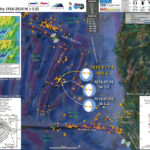
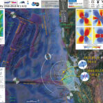
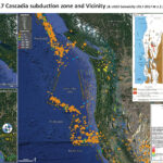
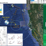
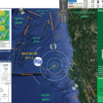
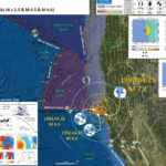
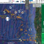
Well, so exciting to have more earthquakes to write about! This summer has been a low seismic summer. The entire year actually.
There was an earthquake within the Gorda plate a few days ago, but these M 5.3 and M 5.6 earthquakes are unlikely to be related, at least in a physical reality sort of way. Here is my Earthquake Report for the Gorda plate earthquake sequence.
This morning (my time) there was an earthquake along the Blanco fracture zone system (BFZ). Today’s earthquake(s) are too small and too far away to directly affect or impact the Cascadia subduction zone megathrust fault. However, I prepare this report because it is a great way to explore the complexities along the BFZ.
The BFZ is a transform plate boundary that connects the Juan de Fuca ridge with the Gorda rise spreading centers. This active fault zone consists of numerous right-lateral (dextral) faults. There is some debate as to how far east the BFZ extends beyond the Gorda rise (some pose it extends far past the trench and ambient noise tomographic data supports this interpretation; Porritt et al., 2011). I remember a colleague of mine who once adamantly stated that there is no evidence for the extension of the BFZ eastwards past the megathrust fault tip. However, this colleague made this statement a decade before the Porritt et al. (2011) data were to be published. My colleague is may still be correct as other experts agree with them.
The interesting thing about today’s M 5.3 earthquake is that it is extensional (normal faulting). This is not altogether unexpected, but interesting nonetheless. Most people might expect the BFZ to have dominantly strike-slip earthquakes. This is largely true, but there are “pull-apart basins” along the BFZ. As strike-slip faults may not be oriented perfectly to the strain field (the tectonic forces driving plate motion and deformation of the lithosphere or crust), other structures may form to accommodate this imperfection. One example of this is a pull apart basin. There are various other causes for pull apart basins too. For example, as faults may bend or change orientation (also in response to the strain field), pull apart basins (or compressional pop up structures) may form.
However, it is possible (probable, given the bathymetric data) that this M 5.3 is not associated with a pull apart basin, but simply the reactivation of a spreading ridge normal fault in response to the complicated tectonics along the BFZ.

Magnetic Anomalies

In the map below, I include a transparent overlay of the magnetic anomaly data from EMAG2 (Meyer et al., 2017). As oceanic crust is formed, it inherits the magnetic field at the time. At different points through time, the magnetic polarity (north vs. south) flips, the north pole becomes the south pole. These changes in polarity can be seen when measuring the magnetic field above oceanic plates. This is one of the fundamental evidences for plate spreading at oceanic spreading ridges (like the Gorda rise).
Regions with magnetic fields aligned like today’s magnetic polarity are colored red in the EMAG2 data, while reversed polarity regions are colored blue. Regions of intermediate magnetic field are colored light purple.
Note that along the Gorda rise, the magnetic anomaly is red, showing that the spreading ridge has a normal polarity, like that of today. Prior to about 780,000 years ago, the polarity was reversed. During the Bruhnes-Matuyama magnetic polarity reversal, the polarity flipped to the way it is today. Note how as one goes away from the Gorda rise (east or west), the magnetic anomaly changes color to blue. At the boundary between red and blue is the Bruhnes-Matuyama magnetic polarity reversal.
The structures in the Gorda, Juad de Fuca, and Pacific plates in this region are largely inherited from the extensional tectonic and volcanic processes at the Gorda rise and Juan de Fuca Ridge. However, the Gorda plate is being pulverized by the surrounding tectonic plates. There are several interpretations about how the plate is deforming and some debate about whether the Gorda plate is even behaving like a plate.
Note how some of the magnetic anomalies appear to be offset along lines that are sub-parallel to the BFZ. This is because they are.

Below is my interpretive poster for this earthquake

I plot the seismicity from the past month, with color representing depth and diameter representing magnitude (see legend). I one version, I include earthquake epicenters from 1918-2018 with magnitudes M ≥ 6.0.
I plot the USGS fault plane solutions (moment tensors in blue and focal mechanisms in orange), possibly in addition to some relevant historic earthquakes.

I placed a moment tensor / focal mechanism legend on the poster. There is more material from the USGS web sites about moment tensors and focal mechanisms (the beach ball symbols). Both moment tensors and focal mechanisms are solutions to seismologic data that reveal two possible interpretations for fault orientation and sense of motion. One must use other information, like the regional tectonics, to interpret which of the two possibilities is more likely.

I include some inset figures.
In the upper right corner is a map of the Cascadia subduction zone (CSZ) and regional tectonic plate boundary faults. This is modified from several sources (Chaytor et al., 2004; Nelson et al., 2004). I placed a blue stars in the general location of today’s earthquake (as in other inset figures in this poster).
In the lower right corner is an illustration modified from Plafker (1972). This figure shows how a subduction zone deforms between (interseismic) and during (coseismic) earthquakes. Today’s earthquake did not occur along the CSZ, so did not produce crustal deformation like this. However, it is useful to know this when studying the CSZ. Today’s earthquakes happened in the lower Gorda plate
In the upper left corner is a map showing the details for the faulting along the BFZ (Braunmiller and Nabelek (2008). Note that this zone is quite complicated and includes several nornal fault bounded pull-apart basins.
In the lower left corner is a map from Dziak et al. (2000) that shows the topography (in the upper panel) and the faulting (in the lower panel) along the BFZ. Blue = lower elevation, deeper oceanic depths; Red = shallower oceanic depth, higher elevation. I placed orange arrows to help one locate the normal faults (perpendicular to the strike-slip faults) in this map. Compare this inset map with the Google Earth bathymetry in the main map. Can you see the BFZ perpendicular ridges?

USGS Earthquake Pages

These are from this current sequence

2018-07-29 M 5.3

These are from earlier

1985-03-13 M 6.5
1994-10-27 M 6.3
2003-01-16 M 6.3
2008-01-10 M 6.3

Here is the map with the seismicity from the past 30 days.

Here is the same map with the seismicity from 1918-2018.

Some Relevant Discussion and Figures

Here is a map of the Cascadia subduction zone, modified from Nelson et al. (2006). The Juan de Fuca and Gorda plates subduct norteastwardly beneath the North America plate at rates ranging from 29- to 45-mm/yr. Sites where evidence of past earthquakes (paleoseismology) are denoted by white dots. Where there is also evidence for past CSZ tsunami, there are black dots. These paleoseismology sites are labeled (e.g. Humboldt Bay). Some submarine paleoseismology core sites are also shown as grey dots. The two main spreading ridges are not labeled, but the northern one is the Juan de Fuca ridge (where oceanic crust is formed for the Juan de Fuca plate) and the southern one is the Gorda rise (where the oceanic crust is formed for the Gorda plate).

Here is a version of the CSZ cross section alone (Plafker, 1972). This shows two parts of the earthquake cycle: the interseismic part (between earthquakes) and the coseismic part (during earthquakes). Regions that experience uplift during the interseismic period tend to experience subsidence during the coseismic period.

This is a diagram that shows how a pull apart basin might form (Wu et al., 2009).

General characteristics of a pull-apart basin in a dextral side-stepping fault system. The pull-apart basin is defined to develop in pure strike-slip when alpha = 0 degrees and in transtension when 0 degrees < alpha 45 degrees.

This figure shows the results of modeling in clay, showing a pull apart basin form (Wu et al., 2009).

Plan view evolution of transtensional pull-apart basin model illustrated with: (a) time-lapse overhead photography; and (b) fault interpretation and incremental basin subsidence calculated from differential laser scans. Initial and final baseplate geometry shown with dashed lines; (c) basin topography at end of experiment.

With these analog models in mind, consider the map below from Braunmiller and Nabelek (2008). This map shows bathymetry (depth in the ocean) in color (units in meters below sea level). They also plot earthquake mechanisms to show how there is extension at the boundary of these basins and strike-slip motion along the strike slip faults. The uncertainty in their locaions are represented by the crosses. I include their figure caption below

Close-up of the BTFZ. Plotted are fault plane solutions (gray scheme as in Figure 10) and well-relocated earthquake epicenters. SeaBeam data are from the RIDGE Multibeam Synthesis Project (http://imager.ldeo.columbia.edu) at the Lamont-Doherty Earth Observatory. Solid and dashed lines mark inferred [Embley and Wilson, 1992] locations of active
and inactive faults, respectively.

Here is a detailed map showing a pull apart basin just to the southwest of today’s M 5.3 (Braunmiller and Nabelek, 2008). I include their figure caption below.

Close-up of the BTFZ-Juan de Fuca ridge-transform intersection. The deep basins are East Blanco Depression (EBD) and West Blanco Depression (WBD); the bathymetric high south of WBD is the Parks Plateau. White arrows are slip vector azimuths of strike-slip events (Figure 16) with tails at their epicenters. Possible active fault strands are shown schematically as solid and dashed lines and are marked (WBDN, WBDC, WBDS, and PPF); solid northerly trending lines illustrate right stepping of (some) transform motion at the EBD.

This is the figure from Dziak et al. (2000) for us to evaluate. I include their long figure caption below.

(Top) Sea Beam bathymetric map of the Cascadia Depression, Blanco Ridge, and Gorda Depression, eastern Blanco Transform Fault Zone (BTFZ).Multibeam bathymetry was collected by the NOAA R/V’s Surveyor and Discoverer and the R/V Laney Chouest during 12 cruises in the 1980’s and 90’s. Bathymetry displayed using a 500 m grid interval. Numbers with arrows show look directions of three-dimensional diagrams in Figures 2 and 3. (Bottom) Structure map, interpreted from bathymetry, showing active faults and major geologic features of the region. Solid lines represent faults, dashed lines are fracture zones, and dotted lines show course of turbidite channels. When possible to estimate sense of motion on a fault, a filled circle shows the down-thrown side. Inset maps show location and generalized geologic structure of the BTFZ. Location of seismic reflection and gravity/magnetics profiles indicated by opposing brackets. D-D’ and E-E’ are the seismic reflection profiles shown in Figures 8a and 8b, and G-G’ is the gravity and magnetics profile shown in Figure 13. Submersible dive tracklines from sites 1 through 4 are highlighted in red. L1 and L2 are two lineations seen in three-dimensional bathymetry shown in Figures 2 and 3. Location of two Blanco Ridge slump scars indicated by half-rectangles, inferred direction of slump shown by arrow, and debris location (when identified) designated by an ‘S’. CD stands for Cascadia Depression, BR is Blanco Ridge, GD is Gorda Depression, and GR is Gorda Ridge. Numbers on north and south side of transform represent Juan de Fuca and Pacific plate crustal ages inferred from magnetic anomalies. Long-term plate motion rate between the Pacific and southern Juan de Fuca plates from Wilson (1989).

BFZ Historic Seismicity

There were two Mw 4.2 earthquakes associated with this plate boundary fault system in mid 2015. I plot the moment tensors for these earthquakes (USGS pages: 4/7/15 and 4/11/15) in this map below. I also have placed the relative plate motions as arrows, labeled the plates, and placed a transparent focal mechanism plot above the BFZ showing the general sense of motion across this plate boundary. There have been several earthquakes along the Mendocino fault recently and I write about them 1/2015 here and 4/2015 here.

There was also seismic activity along the BFZ later in 2015. Here are my report and report update.
Here is a map showing these earthquakes, with moment tensors plotted for the M 5.8 and M 5.5 earthquakes. I include an inset map showing the plate configuration based upon the Nelson et al. (2004) and Chaytor et al. (2004) papers (I modified it). I also include a cross section of the subduction zone, as it is configured in-between earthquakes (interseismic) and during earthquakes (coseismic), modified from Plafker (1972).

I put together an animation that includes the seismicity from 1/1/2000 until 6/1/2015 for the region near the Blanco fracture zone, with earthquake magnitudes greater than or equal to M = 5.0. The map here shows all these epicenters, with the moment tensors for earthquakes of M = 6 or more (plus the two largest earthquakes from today’s swarm). Here is the page that I posted regarding the beginning of this swarm. Here is a post from some earthquakes earlier this year along the BFZ.
Earthquake epicenters are plotted with the depth designated by color and the magnitude depicted by the size of the circle. These are all fairly shallow earthquakes at depths suitable for oceanic lithosphere.

Here is the list of the earthquakes with moment tensors plotted in the above maps (with links to the USGS websites for those earthquakes):

2000/06/02 M 6.0
2003/01/16 M 6.3
2008/01/10 M 6.3
2012/04/12 M 6.0
2015/06/01 M 5.8
2015/06/01 M 5.9

csv file
kml file (not animated)
kml file (animated)

VIDEOS

First Animation (20 mb mp4 file)
Second Animation (10 mb mp4 file)

Here is the first animation that first adds the epicenters through time (beginning with the oldest earthquakes), then removes them through time (beginning with the oldest earthquakes).

Here is the second animation that uses a one-year moving window. This way, one year after an earthquake is plotted, it is removed from the plot. This animation is good to see the spatiotemporal variation of seismicity along the BFZ.

Here is a map with all the fore- and after-shocks plotted to date.

Geologic Fundamentals

For more on the graphical representation of moment tensors and focal mechnisms, check this IRIS video out:

Here is a fantastic infographic from Frisch et al. (2011). This figure shows some examples of earthquakes in different plate tectonic settings, and what their fault plane solutions are. There is a cross section showing these focal mechanisms for a thrust or reverse earthquake. The upper right corner includes my favorite figure of all time. This shows the first motion (up or down) for each of the four quadrants. This figure also shows how the amplitude of the seismic waves are greatest (generally) in the middle of the quadrant and decrease to zero at the nodal planes (the boundary of each quadrant).

There are three types of earthquakes, strike-slip, compressional (reverse or thrust, depending upon the dip of the fault), and extensional (normal). Here is are some animations of these three types of earthquake faults. The following three animations are from IRIS.

Strike Slip:

Compressional:

Extensional:

This is an image from the USGS that shows how, when an oceanic plate moves over a hotspot, the volcanoes formed over the hotspot form a series of volcanoes that increase in age in the direction of plate motion. The presumption is that the hotspot is stable and stays in one location. Torsvik et al. (2017) use various methods to evaluate why this is a false presumption for the Hawaii Hotspot.

A cutaway view along the Hawaiian island chain showing the inferred mantle plume that has fed the Hawaiian hot spot on the overriding Pacific Plate. The geologic ages of the oldest volcano on each island (Ma = millions of years ago) are progressively older to the northwest, consistent with the hot spot model for the origin of the Hawaiian Ridge-Emperor Seamount Chain. (Modified from image of Joel E. Robinson, USGS, in “This Dynamic Planet” map of Simkin and others, 2006.)

Here is a map from Torsvik et al. (2017) that shows the age of volcanic rocks at different locations along the Hawaii-Emperor Seamount Chain.

Hawaiian-Emperor Chain. White dots are the locations of radiometrically dated seamounts, atolls and islands, based on compilations of Doubrovine et al. and O’Connor et al. Features encircled with larger white circles are discussed in the text and Fig. 2. Marine gravity anomaly map is from Sandwell and Smith.

Cascadia subduction zone

General Overview

1700.09.26 M 9.0 Cascadia’s 315th Anniversary 2015.01.26
1700.09.26 M 9.0 Cascadia’s 316th Anniversary 2016.01.26 updated in 2017 and 2018
1992.04.25 M 7.1 Cape Mendocino 25 year remembrance
1992.04.25 M 7.1 Cape Mendocino 25 Year Remembrance Event Page
Earthquake Information about the CSZ 2015.10.08

Earthquake Reports

Social Media

References:

Atwater, B.F., Musumi-Rokkaku, S., Satake, K., Tsuju, Y., Eueda, K., and Yamaguchi, D.K., 2005. The Orphan Tsunami of 1700—Japanese Clues to a Parent Earthquake in North America, USGS Professional Paper 1707, USGS, Reston, VA, 144 pp.
Chaytor, J.D., Goldfinger, C., Dziak, R.P., and Fox, C.G., 2004. Active deformation of the Gorda plate: Constraining deformation models with new geophysical data: Geology v. 32, p. 353-356.
Dengler, L.A., Moley, K.M., McPherson, R.C., Pasyanos, M., Dewey, J.W., and Murray, M., 1995. The September 1, 1994 Mendocino Fault Earthquake, California Geology, Marc/April 1995, p. 43-53.
Dziak, R.P., Fox, C.G., Embleey, R.W., Nabelek, J.L., Braunmiller, J., and Koski, R.A., 2000. Recent tectonics of the Blanco Ridge, eastern blanco transform fault zone in Marine Geophysical Researches, vol. 21, p. 423-450
Frisch, W., Meschede, M., Blakey, R., 2011. Plate Tectonics, Springer-Verlag, London, 213 pp.
Geist, E.L. and Andrews D.J., 2000. Slip rates on San Francisco Bay area faults from anelastic deformation of the continental lithosphere, Journal of Geophysical Research, v. 105, no. B11, p. 25,543-25,552.
Irwin, W.P., 1990. Quaternary deformation, in Wallace, R.E. (ed.), 1990, The San Andreas Fault system, California: U.S. Geological Survey Professional Paper 1515, online at: http://pubs.usgs.gov/pp/1990/1515/
Lin, J., R. S. Stein, M. Meghraoui, S. Toda, A. Ayadi, C. Dorbath, and S. Belabbes (2011), Stress transfer among en echelon and opposing thrusts and tear faults: Triggering caused by the 2003 Mw = 6.9 Zemmouri, Algeria, earthquake, J. Geophys. Res., 116, B03305, doi:10.1029/2010JB007654.
McCrory, P.A.,. Blair, J.L., Waldhauser, F., kand Oppenheimer, D.H., 2012. Juan de Fuca slab geometry and its relation to Wadati-Benioff zone seismicity in JGR, v. 117, B09306, doi:10.1029/2012JB009407.
McLaughlin, R.J., Sarna-Wojcicki, A.M., Wagner, D.L., Fleck, R.J., Langenheim, V.E., Jachens, R.C., Clahan, K., and Allen, J.R., 2012. Evolution of the Rodgers Creek–Maacama right-lateral fault system and associated basins east of the northward-migrating Mendocino Triple Junction, northern California in Geosphere, v. 8, no. 2., p. 342-373.
Meyer, B., Saltus, R., Chulliat, a., 2017. EMAG2: Earth Magnetic Anomaly Grid (2-arc-minute resolution) Version 3. National Centers for Environmental Information, NOAA. Model. doi:10.7289/V5H70CVX
Nelson, A.R., Asquith, A.C., and Grant, W.C., 2004. Great Earthquakes and Tsunamis of the Past 2000 Years at the Salmon River Estuary, Central Oregon Coast, USA: Bulletin of the Seismological Society of America, Vol. 94, No. 4, pp. 1276–1292
Rollins, J.C. and Stein, R.S., 2010. Coulomb stress interactions among M ≥ 5.9 earthquakes in the Gorda deformation zone and on the Mendocino Fault Zone, Cascadia subduction zone, and northern San Andreas Fault: Journal of Geophysical Research, v. 115, B12306, doi:10.1029/2009JB007117, 2010.
Stoffer, P.W., 2006, Where’s the San Andreas Fault? A guidebook to tracing the fault on public lands in the San Francisco Bay region: U.S. Geological Survey General Interest Publication 16, 123 p., online at http://pubs.usgs.gov/gip/2006/16/
Yue, H., Zhang, Z., Chen, Y.J., 2008. Interaction between adjacent left-lateral strike-slip faults and thrust faults: the 1976 Songpan earthquake sequence in Chinese Science Bulletin, v. 53, no. 16, p. 2520-2526
Wallace, Robert E., ed., 1990, The San Andreas fault system, California: U.S. Geological Survey Professional Paper 1515, 283 p. [http://pubs.usgs.gov/pp/1988/1434/].

°
≥

#Earthquake Report: Gorda plate

Posted on July 24, 2018 by Jay Patton

Over the past night and morning, there was a sequence of earthquakes within the Gorda plate due west of Crescent City. Some people even felt these earthquakes, culminating (so far) with a M 5.6. There was a Gorda plate earthquake in March of this year, but it was in a different location.
These earthquakes did not occur along the Gorda Rise as some have reported, but within a region of oceanic crust over a million years old.
In the map below, I include a transparent overlay of the magnetic anomaly data from EMAG2 (Meyer et al., 2017). As oceanic crust is formed, it inherits the magnetic field at the time. At different points through time, the magnetic polarity (north vs. south) flips, the north pole becomes the south pole. These changes in polarity can be seen when measuring the magnetic field above oceanic plates. This is one of the fundamental evidences for plate spreading at oceanic spreading ridges (like the Gorda rise).
Regions with magnetic fields aligned like today’s magnetic polarity are colored red in the EMAG2 data, while reversed polarity regions are colored blue. Regions of intermediate magnetic field are colored light purple.
Note that along the Gorda rise, the magnetic anomaly is red, showing that the spreading ridge has a normal polarity, like that of today. Prior to about 780,000 years ago, the polarity was reversed. During the Bruhnes-Matuyama magnetic polarity reversal, the polarity flipped to the way it is today. Note how as one goes away from the Gorda rise (east or west), the magnetic anomaly changes color to blue. At the boundary between red and blue is the Bruhnes-Matuyama magnetic polarity reversal. The earthquakes from today occurred within this blue region, so the oceanic crust is older than about 780,000 years old, probably older than a million years old.
The structures in the Gorda plate in this region are largely inherited from the extensional tectonic and volcanic processes at the Gorda rise. However, the Gorda plate is being pulverized by the surrounding tectonic plates. There are several interpretations about how the plate is deforming and some debate about whether the Gorda plate is even behaving like a plate. These normal fault (extensional) structures have been reactivating as left-lateral strike-slip faults as a result of this deformation. This region is called the Mendocino deformation zone (a.k.a. the Triangle of Doom).

Below is my interpretive poster for this earthquake

I placed a moment tensor / focal mechanism legend on the poster. There is more material from the USGS web sites about moment tensors and focal mechanisms (the beach ball symbols). Both moment tensors and focal mechanisms are solutions to seismologic data that reveal two possible interpretations for fault orientation and sense of motion. One must use other information, like the regional tectonics, to interpret which of the two possibilities is more likely.

I include some inset figures.
In the upper right corner is a map of the Cascadia subduction zone (CSZ) and regional tectonic plate boundary faults. This is modified from several sources (Chaytor et al., 2004; Nelson et al., 2004). I placed a blue stars in the general location of today’s earthquakes.
In the upper left corner is a map from Chaytor et al. (2004) that shows some details of the faulting in the region. This figure shows the predominant tectonic fabric in the GP (northeast striking left-lateral faults). More about this figure can be found below.
In the lower right corner is a figure from Rollins and Stein (2010). In their paper they discuss how static coulomb stress changes from earthquakes may impart (or remove) stress from adjacent crust/faults. I place a blues star in the general location of today’s earthquakes.
In the lower left corner is a figure from Chaytor et al. (2004) that shows the different models for the internal deformation within the Gorda plate.

This version includes earthquakes M ≥ 5.0 from the USGS. Note how the region where today’s earthquakes happened is a region of higher levels of seismicity. Perhaps this is because this region is the locus of the deformation within the Mendocino deformation zone?