Earthquake Report: Owens Valley, CA

Posted on June 27, 2020 by Jay Patton

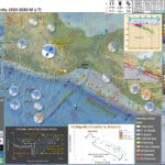
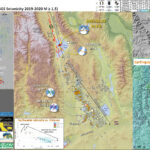
Well, the east side of the Sierra lives up to its reputation for being in earthquake country. From the July 2019 Ridgecrest Earthquake Sequence (reports here)to some shakers east of Mono Lake, to the May 2020 Monte Cristo Earthquake Sequence (report here) to some earthquakes in the Owens Lake area of California. Residents of Olancha, Lone Pine, and Keeler felt strong shaking from a magnitude M 5.8 earthquake, also preceded by about 2 days with a M 4.6 temblor.

https://earthquake.usgs.gov/earthquakes/eventpage/ci39493944/executive

The plate tectonics in the western US is overwhelmingly dominated by the plate boundary between the North America and Pacific plate. The North America plate moves south “relative” to the Pacific plate. Standing on the Pacific plate, looking across the fault, the North America plate moves to your right (a right-lateral strike-slip fault).

Here, both plates are moving “absolutely” in the northwestern direction, but the Pacific plate is moving slower. Therefore the relative sense of motion results in a right-lateral fault.

The plates move side-by-side at a velocity (speed) of about 50 mm per year (2 inches per year). In California, most of this relative motion is localized along the San Andreas fault system. But there are sub-parallel “sibling” faults that also share some of the “slip budget” (their proportion of the 50 mm/yr).

About 20% of the relative plate motion is found along faults on the east side of the Sierra Nevada, along the Eastern California Shear Zone and the Walker Lane system.

Further to the north, in northern California, Oregon, Washington, and Canada, the relative plate motion is compressive, forming the Cascadia subduction zone.

East of California, the plate boundary experiences relative extension, forming the geomorphic province called the Basin and Range. The faults in the Basin and Range are mostly normal faults (extensional faults).
Read more about the different fault types here.

On 26 March 1872 there was a large earthquake that ruptured faults from south of Owens Lake near Olancha, CA northwards to Big Pine, CA. This earthquake may be the largest historic earthquake in California with a magnitude of M 7.8 to 7.9 (Hough and Hutton, 2008).

This earthquake was the result of slip on the Owens Valley fault system (OVF). The majority of slip was right-lateral strike-slip, but because the OVF is not perfectly aligned with the relative plate motion, some of the slip on these faults was normal slip (i.e. extensional).

There are still preserved remains of structures damaged by the earthquake in Lone Pine, CA.

The OVF has been mapped and trenched across to learn about the prehistoric record of earthquakes on the fault.

Also, from measurements of features that have been offset along the fault during earthquakes, along with knowledge of the age of those features, we can estimate how fast the frust is moving relatively across the fault. Below are some figures that help us learn about this historty and activity of the OVF (e.g. Bacon and Pezzopane, 2007; Kirby et al, 2008; Haddon et al., 2013; Bacon et al., 2019).

Beth Haddon et al. (2013) conducted a very interesting study that compiled and updated previous slip estimates for the 1872 OVF earthquake. Their analysis vastly improved the estimate of how much the fault slipped at different locations along the fault (i.e. the fault slip distribution) and included a novel way to account for uncertainty (a.k.a. error) in the measurements of these offsets.

California Geological Survey Engineering Geologist Brian Olson was sent to the field to make observations of fault rupture, landslides, and liquefaction related to this earthquake. Some of his tweets from the field are included below in the social media section.

Below is my interpretive poster for this earthquake

I plot the seismicity from the past month, with diameter representing magnitude (see legend). I include earthquake epicenters from 1920-2020.
I plot the USGS fault plane solutions (moment tensors in blue and focal mechanisms in orange), possibly in addition to some relevant historic earthquakes.
A review of the basic base map variations and data that I use for the interpretive posters can be found on the Earthquake Reports page.
Some basic fundamentals of earthquake geology and plate tectonics can be found on the Earthquake Plate Tectonic Fundamentals page.

I include some inset figures. Some of the same figures are located in different places on the larger scale map below.

In the upper left corner is a map that shows the earthquake faults and historic earthquake locations (epicenters) in the western US. Historic earthquake fault ruptures are mapped as red lines and labeled with their year and magnitude.
In the lower right corner is a map that shows a comparison of the California Geological Survey Shakemap (a model of how strong the ground might shake during the M 5.8 earthquake) and results from online web surveys from peoples’ real observations (i.e. “Did You Feel It?” reports. The colored lines show the boundary between different levels of intensity using the Modified Mercalli Intensity (NNI) scale. The areas are colored relative to the DYFI reports, using the same MMI scale and colors shown on the legend).
In the lower center is an illustration showing how earthquake intensity is higher closer to the earthquake. With distance, the intensity goes down. This is another comparison between the Shakemap models and the DYFI observations.
In the upper right corner is a map that shows the liquefaction susceptibility, or the chance that an area may experience liquefaction during the earthquake. I present a map that also shows the chance that there will be landslides triggered by the earthquake lower in this report. Also, check out social media section to see videos of evidence of these landslides.

Here is the map with a year’s seismicity plotted (and a century in the overview map).
Something to note is that these Owens Lake earthquakes follow some triggered earthquakes that have been going on in the Coso Mountains and to the west of the reservoirs along the Owens River. Following the Ridgecrest Earthquake Sequence, the crust near the fault that slipped flexed like our elastic waist bands. This flexing caused the forces acting on faults withing the crust to increase and decrease in different places. These changes are called changes in static coulomb stress.
According to some studies (see tweets and the Temblor reports related to Ridgecrest), the area to the northwest of Ridgecrest have increased static coulomb stress changes, which increases the chance that faults might slip in those areas.
Guess where these Owens Valley earthquakes are happening? Yup, in an area tha has possibly experienced an increase in stress.

Below is an updated map that shows the aftershocks (and foreshocks) related to the M 5.8 earthquake.
There have only been two earthquakes in the past century that have magnitudes M ≥ 5. Some earthquakes can have aftershocks that last centuries (like the 1872 central Washington earthquake, which is still popping off aftershocks today). Because of the paucity of seismicity in this area, we may not be able to know if these two events in 2009 are aftershocks from 1872. The same is true for the M 5.8 sectence that is ongoing right now in Owens Valley. I suspect that these are unrelated to 1872 and are directly related to the Ridgecrest Earthquakes.
This part of the OVF is at the end of the fault, where it is less organized, so fault lengths are shorter and misaligned. Based on the work of Haddon et al. (2013), the slip on these faults in 1872 was low. So, maybe these faults had more accumulated strain than the rest of the OVF faults, so we would not expect more earthquakes on the OVF system (?). Hard to really know…

I include some inset figures. Some of the same figures are located in different places on the larger scale map below.

In the upper left corner is a map that shows historic earthquake locations (a century M ≥ 2 and a week M ≥ 0). I highlight areas of recent seismic unrest.
In the upper right corner is a map from Bacon et al. (2019) that shows the different faults that they studied in this area. Each different fault is colored and labeled, along with symbology showing what type of relative motion is accommodated on those faults. These authors mapped and dated prehistoric shorelines, then used their location to evaluate slip rates for these faults over a very long time span.
In the lower right corner are some cross sections showing how Bacon et al/ (20219) interpret how the tectonic structures are oriented in the subsurface beneath the Owens Valley. The locations for section A-A’ and B-B’ are shown on the main map as yellow-green lines.

So what does all this mean about the future? We won’t know until the future becomes the present, and then the past.
The Garlock fault south of Ridgecrest. Some of the most detailed paleoseismology studies have taken place along the Garlock fault. Yet, we don’t know if there will be an earthquake there tomorrow or a decade or century from now. Read more about the Garlock fault here.
The Blackwater fault south of Ridgecrest. There are numerous faults in the Eastern California Shear Zone between the Ridgecrest Earthquake Sequence and the Landers and Hector Mine earthquakes from 1992 and 1999 respectively. How do changes in stress following the Ridgecrest earthquake affect the crust south of the Garlock fault? This is a place to watch, but it may take decades, or more, before there is an earthquake here.
The Owens Valley fault north of Ridgecrest. This seems like a lesser likelihood. The average time between large earthquakes on the OVF is several thousands of years and 1972 was the last one. It is possible we don’t know everything about this system (as always, our knowledge about prehistoric earthquakes is a minimum estimate; we may find more evidence later).
The area north of the 1972 OVF earthquake and south of the Cedar Mountain Earthquake or anywhere along the 395 corridor through Walker, Carson City, Reno, etc. The 2019 Pacific Cell Friends of the Pleistocene field trip reviewed some evidences for recent faulting in this region. So, this is a place to watch for sure.

Earthquake Triggered Landslides and Liquefaction

Here is a suite of maps that use USGS earthquake products to help us learn about how earthquakes may affect the landscape: landslide probability and liquefaction susceptibility (a.k.a. the Ground Failure data products)..
First I present the landslide probability model. This is a GIS data product that relates a variety of factors to the probability (the chance of) landslides as triggered by this earthquake. There are a number of assumptions that are made in order to be able to produce this model across such a large region, though this is still of great value (like other aspects from the USGS, e.g. the PAGER alert). Learn more about all of these Ground Failure products here.
There are many different ways in which a landslide can be triggered. The first order relations behind slope failure (landslides) is that the “resisting” forces that are preventing slope failure (e.g. the strength of the bedrock or soil) are overcome by the “driving” forces that are pushing this land downwards (e.g. gravity). I spend more time discussing landslides and liquefaction in this recent earthquake report.
This model, like all landslide computer models, uses similar inputs. I review these here:

Some information about ground shaking. Often, people use Peak Ground Acceleration, though in the past decade+, it has been recognized that the parameter “Arias Intensity” is a better measure of the energy imparted by the earthquake across the land and seascape. Instead of simply accounting for the peak accelerations, AI integrates the entire energy (duration) during the earthquake. That being said, PGA is a more common parameter that is available for people to use. For example, when I was modeling slope stability for the 2004 Sumatra-Andaman subduction zone earthquake, the only model that was calibrated to observational data were in units of PGA. The first order control to shaking intensity (energy observed at any particular location) is distance to the earthquake fault that slipped.
Some information about the strength of the materials (e.g. angle of internal friction (the strength) and cohesion (the resistance).
Information about the slope. Steeper slopes, with all other things being equal, are more likely to fail than are shallower slopes. Think about skiing. Beginners (like me) often choose shallower slopes to ski because they will go down the slope slower, while experts choose steeper slopes.

I use the same color scheme that is presented by the USGS on their website. Note that the majority of areas that may have experienced earthquake triggered landslides are cream in color (0.3-1%). There are a few places with a slightly higher chance that there were triggered landslides. It is possible that there were no significant landslides from this earthquake. The lower bounds for earthquake triggered landslides on land is about M 5.5 and a M 6.4 releases much more energy than that.
Landslide ground shaking can change the Factor of Safety in several ways that might increase the driving force or decrease the resisting force. Keefer (1984) studied a global data set of earthquake triggered landslides and found that larger earthquakes trigger larger and more numerous landslides across a larger area than do smaller earthquakes. Earthquakes can cause landslides because the seismic waves can cause the driving force to increase (the earthquake motions can “push” the land downwards), leading to a landslide. In addition, ground shaking can change the strength of these earth materials (a form of resisting force) with a process called liquefaction.
Sediment or soil strength is based upon the ability for sediment particles to push against each other without moving. This is a combination of friction and the forces exerted between these particles. This is loosely what we call the “angle of internal friction.” Liquefaction is a process by which pore pressure increases cause water to push out against the sediment particles so that they are no longer touching.
An analogy that some may be familiar with relates to a visit to the beach. When one is walking on the wet sand near the shoreline, the sand may hold the weight of our body generally pretty well. However, if we stop and vibrate our feet back and forth, this causes pore pressure to increase and we sink into the sand as the sand liquefies. Or, at least our feet sink into the sand.
Below is the liquefaction susceptibility map. I discuss liquefaction more in my earthquake report on the 28 September 20018 Sulawesi, Indonesia earthquake, landslide, and tsunami here.
I use the same color scheme that the USGS uses on their website. Note how the areas that are more likely to have experienced earthquake induced liquefaction are in the valleys. The fact that this earthquake happened in the summer time suggests that there may not have been any liquefaction from this earthquake.

Other Report Pages

Some Relevant Discussion and Figures

Here is a figure from Rinke et al. (2012) that shows the global and regional tectonics here. I include the figure captions below as blockquotes. The first map shows the plate boundary scale tectonic regions. This is a generalized map (e.g. don’t pay attention to where the San Andreas and Cascadia faults are located).

Simplified tectonic map of the western U.S. Cordillera showing the modern plate boundaries and tectonic provinces. Basin and Range Province is in medium gray; Central Nevada seismic belt (CNSB), eastern California shear zone (ECSZ), Intermountain seismic belt (ISB), and Walker Lane belt (WLB) are in light gray; Mina deflection (MD) is in dark gray.

Here is the Amos et al. (2013) plate tectonic map. Check out the location of the historic surface rupturing earthquakes. Their figure caption is below (as for other figures here).

Overview of active faults and regional topography of the Eastern California shear zone (ECSZ) and southern Walker Lane belt. Labeled faults are abbreviated as follows: ALF—Airport Lake fault, BF—Blackwater fault, GF—Garlock fault, KCF—Kern Canyon fault, LLF—Little Lake fault, OVF—Owens Valley fault, SNFF—Sierra Nevada frontal fault. OL—Owens Lake, IWV—Indian Wells Valley. Major historical earthquake surface ruptures in the Eastern California shear zone and Walker Lane belt are outlined in white, with stars denoting epicentral locations: OV—1872 Owens Valley, L—Landers 1992, HM—1999 Hector Mine. Active fault traces are taken from the U.S. Geological Survey Quaternary fault and fold database, with the exception of the Kern Canyon fault, taken from Brossy et al. (2012).

This map extends a little farther to the east (Frankel et al., 2008). This map shows nicely how the Sierra Nevada and Owens Valley faults (the Pacific-North America plate boundary) and Eastern California Shear Zone, aka ECSZ (the maps south of the Garlock fault, 35.5N°) interact with east-west trending left-lateral strike-slip faults like the Garlock fault. The ’92 Landers and ’99 Hector Mine Earthquakes are on faults in the ECSZ.

Shaded relief index map of Quaternary faults, roads, towns, and fi eld trip stops in the eastern California shear zone. Most faults are from the U.S. Geological Survey Quaternary fault and fold database (http://earthquake.usgs.gov/regional/qfaults). Arrows indicate relative fault motion for strike slip faults. Bar and circle indicates the hanging wall of normal faults. Field trip stop location numbers are tied to site descriptions in the fi eld guide section. AHF—Ash Hill fault; ALF—Airport Lake fault; B—Bishop; BF—Blackwater fault; BLF—Bicycle Lake fault; BM—Black Mountains; BP—Big Pine; Br—Baker; Bw—Barstow; By—Beatty; CA—California; CF—Cady fault; CLF—Coyote Lake fault; CoF—Calico fault; CRF—Camp Rock fault; DSF—Deep Springs fault; DV-FLVF—Death Valley–Fish Lake Valley fault; EPF—Emigrant Peak fault; EV— Eureka Valley; FIF—Fort Irwin fault; FM—Funeral Mountains; GF—Garlock fault; GFL—Goldstone Lake fault; GM—Grapevine Mountains; HF—Helendale fault; HLF—Harper Lake fault; HMSVF—Hunter Mountain–Saline Valley fault; I—Independence; LF—Lenwood fault; LLF— Lavic Lake fault; LoF—Lockhart fault; LP—Lone Pine; LuF—Ludlow fault; LV—Las Vegas; M—Mojave; MF—Manix fault; NV—Nevada; O—Olancha; OL—Owens Lake; OVF—Owens Valley fault; P—Pahrump; PF—Pisgah fault; PV—Panamint Valley; PVF—Panamint Valley fault; R—Ridgecrest; S—Shoshone; SAF—San Andreas fault; SDVF—southern Death Valley fault; SLF—Stateline fault; SPLM—Silver Peak–Lone Mountain extensional complex; SNF—Sierra Nevada frontal fault; SP—Silver Peak Range; T—Tonopah; TF—Tiefort Mountain fault; TMF—Tin Mountain fault; TPF—Towne Pass fault; WMF—White Mountains fault; YM—Yucca Mountain.

This is also from Amos et al. (2013) that shows how some northeast striking normal faults are related to the Little Lake fault, in the northern part of Indian Wells Valley. The Little Lake fault connects to the Sierra Nevada frontal fault.

Simplified geologic map of the Little Lake fault, highlighting Quaternary volcanic and alluvial deposits bearing on the Pleistocene drainage of Owens River through the Little Lake area. Map units are named and modified from Duffield and Bacon (1981). The 30 m elevation contours are taken from the National Elevation Database (NED). The ⁴⁰Ar/³⁹Ar dates are labeled as in Table 1. SNFF—Sierra Nevada frontal fault.

Here is the Frankel et al. (2008) larger scale fault map, also focusing on the northern Indian Wells Valley.

Northward branching of the Holocene-active Airport Lake fault zone in northern Indian Wells Valley, Rose Valley, the Coso Range, and Wild Horse Mesa. AL—Airport Lake playa; BR— basement ridge; CB—Central branch; CWF—Coso Wash fault; EB—Eastern branch; GF—geothermal field; HS— Haiwee Spring; LCF—Lower Cactus Flat; MF—McCloud Flat; UCF—Upper Centennial Flat; WB—Western branch; WHA—White Hills anticline; WHM—Wild Horse Mesa; WHMFZ— Wild Horse Mesa fault zone. Faults with especially prominent scarps in Wild Horse Mesa are highlighted in bold. Late Quaternary faults modified from Duffield and Bacon (1981) and Whitmarsh (1998), with additional original mapping. A and B indicate two faults that display evidence for late Quaternary dextral offset.

This is the Stevens et al. (2013) map that shows the sedimentary basins in the region.

Map showing interpreted thickness of Cenozoic deposits and major faults outlining the deep basins, based on inversion of gravity data [56]. Connection between West Inyo and Southwest Argus faults from Pluhar et al. [58]. ALFZ = Airport Lake Fault Zone; CWF = Coso Wash Fault; EIF = East Inyo Fault; LLF = Little Lake Fault. A-A’ to H-H’ indicate lines of cross sections and gravity profiles shown in Figure 10.

Here are the fault blocks presented by Stevens et al. (2013).

Map showing deep basins, relatively shallow down-dropped blocks, extended mountain blocks, and structural zones in the ESVS, which is bounded by largely unextended mountain blocks. CB = Chalfant Basin; NBB = North Bishop Block; RVB = Round Valley Basin

Here is a great overview map of the faults in the region from Oskin et al. (2008). Their paper is about their research to quantify the tectonic loading of faults in the Eastern California shear zone. Note that they use about 12 mm per year of Pacific-North America relative plate motion across this region.

A: Index map of southwest North America showing geodetic provinces from Bennett et al. (2003) and location of Mojave block. Velocities of geodetically stable regions are shown relative to Colorado Plateau. ECSZ—eastern California shear zone in Mojave block. Shear zone continues northward into western Great Basin province. GF—Garlock fault. B: Index map of the Mojave block with active faults and locations of recent earthquake ruptures. Circles show localities of slip-rate measurements that sum to ≤6.2 ± 1.9 mm/yr across the ECSZ. GPS—global positioning system.

Here is another good overview map, showing the faults for which Petersen and Wesnousky (1994) reviewed slip rates in that publication. They present an excellent review of all slip rate and paleoseismic investigations at the time that paper was published.

Map showing sites of slip rate studies in southern California for the San Andreas (SAI-14), San Jacinto (SJI-13), Elsinore-Whittier (El-8), Newport- Inglewood (N1-3), Palos Verdes (N4-6), Rose Canyon (N7), Transverse Ranges (T1-50), Mojave (MI-6), and Garlock (G1-9) faults.

Oskin and Iriondo studied the Blackwater fault, the right-lateral strike-slip fault system that extends from the south into the region of the Ridgecrest Earthquake Sequence. The Blackwater fault is connected to the south with the Calico fault (a fault between the 1992 and 1999 earthquakes). This appears to be the major Eastern California Shear zone fault that extends towards the Airport Valley and Little Lake faults (which ruptured during the Ridgecrest Earthquake Sequence).

A: Index map of Pacific–North America plate boundary through southwest North America. Principal faults are shown as thick black lines. Tectonically stable areas are outlined by dotted lines. Walker Lane and Eastern California shear zone, shown as dark gray band encompassing network of active faults, together absorb 9%–23% of total plate boundary shear (Dixon et al., 2000; Dokka and Travis, 1990a). JDF—Juan de Fuca; MTJ— Mendocino triple junction. B: Index map of Eastern California shear zone showing fault slip rates (in parentheses, mm/yr) determined by paleoseismic studies (Klinger and Piety, 2000; Lee et al., 2001; McGill and Sieh, 1993; Rockwell et al., 2000; Zhang et al., 1990). Heavy dark gray lines outline historic earthquake ruptures (Beanland and Clark, 1994; Sieh et al., 1993; Treiman et al., 2002). Heavy, medium gray band highlights Blackwater–Calico fault system. Light gray band surrounding Blackwater fault and passing north of Garlock fault is zone of localized 1.2 6 0.5 mm/yr strain accumulation documented by radar interferometry (Peltzer et al., 2001). C: Neotectonic map of Blackwater fault, showing type and orientation of fault line scarps with ticks on downthrown side. Dark patterned areas are lava flows cut by Blackwater fault (Dibblee, 1968, 1967; Smith, 1964)

Peltzer et al. (2001) evaluate the amount of tectonic strain that has accumulated over time (see geodesy section to learn more about strain). First I present their tectonic map.

Tectonic map of southern California. Solid lines are active faults (Jennings, 1975). Yellow dots are relocated earthquakes between 1981 and 2000 (Hauksson, 2000). Dashed-line box is area covered by Earth Resource Satellite (ERS) data used in this study. White dashed line shows location of concentrated shear observed in synthetic aperture radar (SAR) data. Black stars indicate epicenters of recent earthquakes: OV—1872 Owens Valley, JT—1992 Joshua Tree, L—1992 Landers, BB—1992 Big Bear, N—1994 Northridge, RC—1994 and 1995 Ridgecrest, HM—1999 Hector Mine. Heavy solid lines depict surface ruptures of Landers (Sieh et al., 1993), Hector Mine (U.S. Geological Survey and California Division of Mines and
Geology, 2000; Peltzer et al., 2001), and Owens Valley (Beanland and Clark, 1994; only southern half of rupture is shown) earthquakes. Black dots and arrows show locations and observed velocities of 11 stations of Yucca GPS array (Gan et al., 2000).
* Faults are listed in the paper

Here is the Guest et al. (2003) map showing their interpretation of how these faults developed over time.

In this model the Owlshead and southern Panamint blocks are hypothesized to have undergone sinistral transtension in response to a clockwise rotation of their southern confining boundary (Garlock fault zone).
RTR—Radio Tower Range, SOM—Southern Owlshead Mountains, WWFZ—WingateWash fault zone, BMF—Brown Mountain fault, OLF—Owl Lake fault, GF—Garlock fault, MSS—Mule Springs strand, LLZ—Leach Lake fault zone, SDVFZ—Southern Death Valley fault zone.

Background Literature – Geodesy

Gan et al. (2003) present a summary of geodetic data where they show that the Owens Valley, Little Lake, and Helendale faults form the generalized western boundary of the Eastern California shear zone (there are additional right-lateral faults to the west however).

Map showing the location of the ECSZ, the GPS arrays, the station velocities (relative to the fixed North America), and the principal faults in southern California (from Jennings [1992]). The thick dashed lines directed N23°W show the boundaries of the assumed parallel-sided ECSZ. The thin dashed lines extended from the segments of the Garlock fault show the trends of the segments.

One of the challenges with interpreting geodetic data is comparing earthquake fault slip rates inferred from geodetic methods with rates calculated using geologic data (either from long term offsets of bedrock, or from more recent rates using fault trenches).
Chuang and Johnson (2011) present their comparisons of GPS slip rates with geologic rates.

Blue = geologic rate
Black = geodetic rate
Magenta = block model rate from their analyses

Comparison of geologic fault slip rates (blue, mm/yr) used in model, range of estimates from elastic block models (black) of Becker et al. (2005) and Meade and Hager (2005), and estimates from our block model (magenta) along major faults. Negative is left lateral. Light red lines are surface fault traces, and white thick lines are model blocks. Blue arrows are Southern California Earthquake Center (SCEC) crustal motion map 3 (Shen et al., 2003) velocities with respect to stable North America.
*See their paper for fault abbreviations.

Here is an interesting figure showing their (Chuang and Johnson, 2011) estimate of the relative position in the earthquake cycle for these faults. This is based on published recurrence intervals for these faults (the average time between earthquakes given paleoseismic investigation data).

Summary of assumed geologic rates, recurrence interval (T), and time since last earthquake (teq) in Southern California. (For further discussion of sources of T and teq, see footnote 1). Blue numbers are expert opinion slip rates from Working Group on California Earthquake Probabilities (2008) and red numbers are rates from other paleoseismology data.
Color of rupture segment represents ratio of time since last earthquake and recurrence interval. Hot (red) colors show segments are in early earthquake cycle, and cold (blue) colors show late earthquake cycle.

This is the summary of the Chuang and Johnson (2011) slip rate comparison.

A: Geologic fault slip rates versus slip rates inferred from geodetic data. Geologic rates are summarized in Table DR1 (see footnote 1). Blue bars are slip rate comparisons from Meade and Hager (2005) and red bars are from this study. B: Normalized velocity across Garlock fault (blue), Mojave segment of San Andreas fault (red), and eastern California shear zone (ECSZ, green) from our cycle model. Black line is normalized velocity derived from elastic model.

Here is an earlier analysis comparing geodetic rates with geologic rates (Dixon et al., 2003). First we see a map showing the faults from which the fault comparisons are shown.

Sketch map of study area, modified from Dixon et al. (1995). Bar marks approximate location of Global Positioning System transect (Gan et al., 2000). GF— Garlock fault. Labeled faults of Eastern California shear zone: ALF— Airport Lake fault zone; OVF—Owens Valley fault zone; HMF—Hunter Mountain–Panamint Valley fault zone; DVF— Death Valley–Furnace
Creek fault zone; FLV— Fish Lake Valley fault zone.

Here is the east west profile from Dixon et al. (2003). The horizontal axis is distance and the vertical axis is the rate that each site moves in mm per year. Their fault modeling is represented by the dark black line.

Global Positioning System velocity (triangles) and one standard error (bars) from Gan et al. (2000) compared to prediction of viscoelastic coupling model (heavy solid line), representing summed velocity contributions from four parallel faults (light dashed lines). SAF—San Andreas fault; DVF—Death Valley–Furnace Creek fault zone; HMF—Hunter Mountain–Panamint Valley fault zone; OVF—Owens Valley fault zone. Inset shows model rheology for Eastern California shear zone. SNB—Sierra Nevada block;B&R— Basin and Range Province; h is fault depth (depth of elastic layer) for three faults (a, b, or c), m is rigidity, h is viscosity. Arrows mark location of major shear-zone faults.

Peltzer et al. (2001) use synthetic aperture radar interferometry (see my second update report for more on InSAR anslysis) to measure tectonic deformation that accumulated between 1992-2000.
The Coso Geothermal Field is the rainbow area in the northernmost part of the map. Indian Wells Valley is the green area to the south of the Coso Field. This is an area of elevated strain. The Garlock fault is the ~east-west black line in the center of the white inset box.

Surface velocity map obtained by averaging 25 interferograms of Los Angeles–Mojave region. One color cycle depicts 10 mm/yr of surface displacement along radar line of sight (at lat N348; ERS [Earth Resource Satellite] descending track trends S13.68W, radar looking westward at 238 off vertical incidence angle in middle of imaged swath). Gray areas are zones of low phase coherence that have been masked in processing. Black lines are active faults (Jennings, 1975). White box indicates subset of synthetic aperture radar (SAR) data that was used for profile in Figure 4. Note conspicuous shear strain along San Andreas fault and shear zone parallel to Blackwater–Little Lake fault system. Large deformation signal in northwest corner of frame is ground subsidence related to Coso volcanic and geothermal field (Fig. 1). Surface displacement associated with 1994 and 1995 Ridgecrest earthquakes is visible south of Coso area. Other patterns of surface deformation include ground subsidence due to groundwater withdrawal in Los Angeles and Lancaster areas (Fig. 1) and to seasonal change of water table level around dry lakes.

Peltzer et al. (2001) plot observations from their radar data showing relative plate motion associated with dislocation along the Blackwater-Little Lake fault system.

Profiles of observed and modeled line-of-sight displacement projected on vertical plane perpendicular to shear zone. Gray dots are individual data points for all radar-image pixels included in box shown in Figure 3. Solid line shows 2 km running mean of observed displacement along profile length. Note that apparent standard deviation of projected data relative to average profile reflects in part displacement gradient parallel to fault strike and not only error in data. Groups of dots that deviate from dense part of profile are due to ground subsidence near lake shores and to surface displacement associated with Ridgecrest earthquakes (Figs. 1, 3). Short-dash line is profile predicted by long-term velocity model used to estimate interferometric baseline (Shen et al., 1996). Long-dash line is profile predicted by velocity model, including additional buried dislocation along Blackwater–Little Lake fault system. Parameters of added fault are given in text. Black dots and error bars (2s) are line-of-sight projections of horizontal velocities observed by GPS at stations of Yucca transect (Gan et al., 2000).

Background Literature – Owens Valley fault

Kylander-Clark et al. (2005) use the lateral offset of plutonic dikes (igneous rocks) to constrain a long term slip rate across the Owens Valley fault. This map shows one of the dike pairs used in their analysis. By knowing the age of these dieks, and the distance that they have been offset, we can obtain a slip rate.

Locations of the Golden Bear and Coso dikes, adjacent to Owens Valley. Main figure shows the Golden Bear and Coso dikes striking into the valley, where they intrude 102 Ma plutons. Both the dikes and the plutons provide distinctive markers that can be matched across the valley and are consistent with 65 km of dextral displacement since 84 Ma. Inset shows other markers across Owens Valley that earlier workers suggested indicate from 0 to 65 km of dextral offset across the valley. Also shown are the traces of the Tinemaha fault (Stevens et al., 1997; Stevens and Stone, 2002) and intrabatholithic break 3 (IBB3; Kistler, 1993), which are hypothesized to accommodate offset of these markers. Note that the section of IBB3 between 38°N and 36.5°N is correlative with the eastern intrabatholithic break (EIB) of Saleeby and Busby (1993). Not all known locations of Independence dikes are indicated. Instead, patterned areas show only the densest parts of the dike swarm as defi ned by Glazner et al. (2003). AR—Argus Range; CR—Coso Range; IR—Inyo Range; WM—White Mountains

Bacon and Pezzopane used trench excavations across earthquake faults to construct a prehistoric earthquake history for the Owens Valley fault. Below is their tectonic map for the region.

(A) Map of major Quaternary faults in the northern Eastern California shear zone and southern and central Walker Lane, as well as the locations of the Owens Valley fault. Faults are modified from Reheis and Dixon (1996) and Wesnousky (2005)
(B) Generalized fault and geology map of south-central Owens Valley, showing the A.D. 1872 Owens Valley fault rupture and major fault zones in the valley (modified from Hollett et al. [1991] and Beanland and Clark [1994]).
(For fault abbreviations, see their paper.)

This map shows a more detailed view of the Owens Valley fault and the Owens Lake topography (Bacon and Pezzopane, 2007).

Shaded relief map of southern Owens Valley showing fault zones and the ages of the most recent prominent highstands and recessional shorelines of Owens Lake during the latest Quaternary (modified from Bacon et al., 2006).

This map shows the Bacon and Pezzopane (2007) field sites.

Map of the field area and locations of paleoseismic study sites in relation to the A.D. 1872 Owens Valley earthquake fault trace near Lone Pine. Study sites are located on the Alabama Hills (AHS), Diaz Lake (DLS), and Manzanar (MZS) sections of the Owens Valley fault zone mapped by Bryant (1988) and Beanland and Clark (1994) from 1:12,000 aerial photographs.

An essential part of any earthquake fault investigation is knowledge about the geologic units that are offset by the fault. Bacon and Pezzopane (2007) also described and interpreted the sediment stratigraphy in southern Owens Valley as part of their research.

Schematic composite stratigraphic column. The generalized stratigraphic and geochronologic relations, developed from exposures at the Alabama Gates and Quaker paleoseismic sites and Owens River bluffs near Lone Pine (Bacon et al., 2006), show the positions of radiocarbon dates, sequence boundaries, and event chronologies as discussed in the text.

The geologic method (McCalpin, 1996) is based on the offset of geologic materials like sedimentary deposits or bedrock lithologic units. Below are trench logs showing the geologic units that Bacon and Pezzopane (2007) use to infer an earthquake history. Geologic evidence is “primary” evidence for earthquakes.

Here is a time series showing the sedimentary and earthquake history as interpreted by Bacon and Pezzopane (2007).

Schematic depiction of stratigraphy and structural relations at the Quaker paleoseismic site prior to the penultimate event and after the A.D. 1872 earthquake (depictions A–H). The stratigraphy and structure exposed in trench T5 (Fig. 7) was retrodeformed and reconstructed one event at a time (while also accounting for other stratigraphic and
paleoseismic relations exposed in adjacent fault trenches and stratigraphic pits). The locations of sequence boundaries (SB0–SB4) are shown and can be referenced on Figure 5.

Haddon et al. (2013) compiled fault offset measurements and presented a summary here, showing the slip distribution along the fault (along strike). The measurements plotted below represent measurements of offsets of features as measured in high resolution LiDAR topographic data. They separate data into lateral offset (the amount of strike-slip relative motion) and throw offset (the amount of normal relative motion, from extension).
We can see that the fault has both strike-slip and normal offsets, with strike-slip the dominant relative motion.

Compilation of small geomorphic offsets measured from lidar using LaDiCaoz_v2 along average OVF strike (3408) (supporting information Tables S2 and S3). Data include confidence ratings of low-moderate to high and omit net values determined by summing. Gray error bars show uncertainty limits determined visually from back-slipping. (a) The spatial distribution of OVF scarps (red lines) mapped from EarthScope lidar and classified by Owens Valley fault section (orange and black points), following previous mapping by Beanland and Clark [1994], Bryant [1984a, 1984b], and Slemmons et al. [2008]. Nearby faults are taken from the U.S. Geological Survey Quaternary fault and fold database. From south to north: DS, Dirty Socks; OL, Owens Lake; LP, Lone Pine fault; DL, Diaz Lake; IS, southern Independence; MF, Manzanar fault; I, Independence; T, Tinemaha; TW, western Tinemaha; FS, Fish Springs; BP, Big Pine; K, Keough section of Sierra Nevada frontal fault (SNNF), KLF, Klondike Lake fault; KSF, Klondike Springs fault; WMF, White Mountain fault. (b) Right-lateral offset measurements symbolized by fault section include previously reported values (orange diamonds) from Bateman [1961], Lubetkin and Clark [1988], Beanland and Clark [1994], Lee et al. [2001a], Zehfuss et al. [2001], and Slemmons et al. [2008]. (c) Along-strike compilation of measured vertical throw. Throw is predominantly east-down, with negative values indicative of downward motion to the west.

This is a spectacular plot showing the along-strike variation in offset measurements.

Frequency distributions and cumulative offset probability density (COPD) plots for lateral and vertical offsets, compiled using bin sizes of 1 and 0.25 m, respectively (supporting information Tables S2 and S3). Histograms omit uncertainties, whereas COPD plots incorporate PDFs generated by the cross-correlation routine and truncated based on the range of uncertainty from back-slipping. Data are color-coded according to major sections of the OVF. (a) Scarps along the southern, central, and northern sections of the OVF relative to volcanic flows (purple) and a few representative elevation contours, generally corresponding to recognized pluviallacustrine features (#1–4) [Bacon et al., 2006; Jayko and Bacon, 2008; Bacon et al., 2013; Bacon et al., 2014]. Age estimates for features documented near (1) 1180 m, (2) 1162 m, (3) 1131 m, and (4) 1101 m are 160632 ka [Jayko and Bacon, 2008], 23,230–26,250 cal yr BP [Bacon et al., 2006], 15,870–16,230 cal yr BP [Bacon et al., 2014], and 300630 to 400630 yr BP [Bacon et al., 2013], respectively. Green points mark surface slip measurements based on geomorphic features. CM, Crater Mountain. Volcanic flows are from the California Geological Survey. (b–e) Optimum offset values for the southern (yellow), central (blue), and northern (red) sections are grouped and shaded by confidence rating. COPD plots use moderate to high confidence offsets and incorporate summed values.

Here is the plot from Haddon et al. (2013) that shows a summary of their displacement measurements from the Owens Valley and Lone Pine faults. The lower panel shows these measurements combined.

Net 1872 surface slip derived from moderate to high confidence displacements plotted along subparallel strands. Gray bars reflect aggregated uncertainties from back-slipping of lidar imagery. (a) Along-strike compilation of displacement values for main traces of the OVF, as predicted by binned COPD plots. (b) Along-strike compilation of Lone Pine fault displacements. (c) Summed distributions (red lines) for possible net 1872 surface slip along a simplified
fault plane striking 3408 and dipping 808 northeast. The maximum implied displacement is between 7 and 11 m and reflects the average of four high values. The net slip averages 4.461.5 m based on a 5-km binned average that incorporates graphical values for gaps between higher confidence data.

Here is their summary map showing slip rates for each of the faults used in their study (Haddon et al., 2013).

Compilation of reported slip rates in mm/yr on active faults in the southern Walker Lane (modified from Foy et al. [2012]) with rspect to the geodetic rate across the zone derived from the global positioning system and the relative motion of the Sierra Nevada– Great Valley microplate [Lifton et al., 2013]. Geologic slip rate studies, from south to north: Amos et al. [2013b], (this study), Oswald and Wesnousky [2002], Frankel et al. [2007a,b], Lubetkin and Clark [1988], Reheis and Sawyer [1997], Lee et al. [2001b], Ganev et al. [2010], Kirby et al. [2006], and Nagorsen-Rinke et al. [2013]. Faults listed alphabetically: AHF, Adobe Hills fault; ALF, Airport Lake fault; BMF, Black Mountain fault; DSF, Deep Springs fault; FCF, Furnace Creek fault; FLVF, Fish Lake Valley fault; HMF, Hunter Mountain fault; LLF, Little Lake fault; OVF, Owens Valley fault; NDVF, Northern Death Valley fault; PVF, Panamint Valley fault; QVF, Queen Valley fault; SAF, San Andreas fault; SNFF, Sierra Nevada frontal fault; SVF, Saline Valley fault; WMF, White Mountain fault.

Dr. Steve Bacon was first infected with the quest for knowledge about the tectonics of the Owens Valley when he attended the 1997 Pacific Cell Friends of the Pleistocene field trip to Owens Valley. IF anyone has a scan of the 1997 Owens Valley guidebook, please contact me.
Dr. Bacon chose to study the Owens Valley fault for his Masters Thesis work at Humboldt State University, Department of Geology. I was lucky enough to help him do some of this work as I was also attending HSU at the time. I also remembering how another researcher had failed to listed to Steve, yet they published a paper where they measured post-earthquake features as it they were offset during the earthquake. The peer review process is imperfect sometimes.
Being a sediment stratigrapher, I appreciate the fact that the key preface to consducting a paleoseismic investigation is developing knowledge about the stratigraphy in the region. This was a major part of Dr. Bacon’s research. Please read more about his analysis of the lake level variations for the past 50,000 years in the Owens Lake in his recently published article (Bacon et al., 2020) listed in the references.
Here is the Bacon et al. (2019) overview map that shows the spatial extent of the 1872 Owens Valley fault earthquake rupture.

Map of primary faults and rocks of the Big Pine volcanic field in south-central Owens Valley. The A.D. 1872 Owens Valley fault rupture and fault segments of the OVF and SNFF are shown (modified from Bacon and Pezzopane, 2007). Faults: CFF—Centennial Flat fault; KF—Keeler fault; ORF—Owens River fault; SFF—Sage Flat fault. Numbers show sites on OVF referred to in text of: 1—Kirby et al. (2008); 2—Lee et al. (2001); and 3—Bacon and Pezzopane (2007).

Here is a map showing the detailed faults in the Owens Lake area, which is the focus of their study (Bacon et al., 2019). These authors used the geometric position of geomorphic features (like shorelines), along with numerical ages of those features (the time that they formed), to calculate long term slip rates for these faults.

Map of primary faults in Owens Lake basin and elevations of deformed shoreline features (∼1156–1166 m) used to estimate the magnitude of ground deformation and slip rates across faults in the lake basin. Faults are modified after Bacon et al. (2005) and Slemmons et al. (2008). Faults: CFF—Centennial Flat fault; COLF—Central Owens Lake fault; IMF—Inyo Mountains fault; KF—Keeler fault; ORF—Owens River fault; OVF—Owens Valley fault; SIMF—southern Inyo Mountains fault; and SNFF—Sierra Nevada frontal fault. The location of the Sage Flat fault (SFF) after Jayko (2009) and Amos et al. (2013a) is also shown. Plunging anticlines from Frankel et al. (2008). Reference elevation contours at 1096 and 1160 m represent the margin of Owens Lake playa and the approximate location of ca. 40.0 ka shoreline features, respectively. Modern sill is also shown relative to the 1160 m elevation that defines the overflow channel of the basin. Sediment lake core OL92 of Smith and Bischoff (1997) is shown relative to the depocenter area of the lake basin. Approximate location of transect for repeat leveling surveys near Lone Pine of Savage and Lisowski (1980, 1995) is also shown. K—town of Keeler; S—Swansea embayment; O—town of Olancha.

This is a summary of fault characteristics as presented by Bacon et al. (2019). Dip-slip rate is the slip rate as measured up and down along the fault (in the direction that water would drip if it were placed on the fault). The extension rate is the slip rate measured horizontally in the same direction.

Here is another map of the Owens Lake area, showing these slip rates and cross section locations for sections shown below (Bacon et al., 2019).

Generalized fault map of Owens Lake basin showing slip rates from this study and previous investigations. Faults: CFF—Centennial Flat fault; COLF—Central Owens Lake fault; IMF—Inyo Mountains fault; KF—Keeler fault; ORF—Owens River fault; OVF—Owens Valley fault; SFF—Sage Flat fault; SIMF—southern Inyo Mountains fault; SNFF—Sierra Nevada frontal fault. Extension direction at N72°E normal to Owens Valley is shown with geologic extension rate from this study and geodetic extension rates from trilateration networks in the valley (Savage and Lisowski, 1995) and GPS arrays across northern Owens Valley (Ganev et al., 2010a). The location of transects A–A′, B–B′, and C–C′ used in cross sections are shown. K—town of Keeler; S—Swansea embayment.

Here are the cross sections showing the faults as these authors (Bacon et al., 2019) interpret their geometry in the subsurface.

Cross sections showing orientation of faults and sense of slip, and reconstructed water levels of the ca. 40 ka highstand pluvial lake in Owens Lake basin. Faults: CFF—Centennial Flat fault; COLF—Central Owens Lake fault; IMF—Inyo Mountains fault; KF—Keeler fault; ORF—Owens River fault; OVF—Owens Valley fault; SFF—Sage Flat fault; SIMF—southern Inyo Mountains fault; SNFF—Sierra Nevada frontal fault. Fault orientations are apparent dip based on fault strike across transects. Inferred locations of IMF and SIMF on transect A–A′ are from Pakiser et al. (1964) and Bacon et al. (2005).

Here is a figure that shows a summary of their analysis (Bacon et al., 2019). Read the caption below to help yourself to understand this figure. It is complicated, but simple at the same time. Read their paper to learn more about this comprehensive and amazing research.

Plots showing the elevation of: (A) deformed ca. 40 ka shoreline features and lowstand beach ridge deposits, and (B) ca. 15 cal k.y. B.P. shorelines features and deformed fluvial-deltaic deposits. The elevation of shoreline features and deposits are projected onto transect B–B′ and shown in relation to the generalized location of faults in Owens Lake basin (Fig. 9). Magnitude of ground deformation shown is ∼10 m subsidence relative to the ca. 40 ka reconstructed water level (i.e., paleohorizontal datum) and ∼3.6 m fault separation on the Keeler fault of the ca. 40 ka beach ridge crests. The elevation and age of fluvial deltaic deposits on the hanging wall of the Owens Valley fault are from paleoseismic fault trench data (Bacon and Pezzopane, 2007). Faults: CFF—Centennial Flat fault; COLF— Central Owens Lake fault; KF—Keeler fault; ORF—Owens River fault; OVF—Owens Valley fault; SIMF—southern Inyo Mountains fault; NFF—Sierra Nevada frontal fault. Actual dips of faults are not shown. Vertical sense of slip is indicated by arrows. Lateral slip is indicated by crosses (away) and dots (toward). The elevation errors from GPS survey of shoreline features and deposits are less than width of symbols.

Background Literature – Earthquake History

Here are the results of the paleoseismic (prehistoric earthquake history) investigation for the Owens Valley fault (Bacon and Pezzopane, 2007).

Fault segmentation and section map of central and southern Owens Valley showing overlap and possible distributive faulting and linkage between the northern segment of the Owens Valley fault (OVF) and southern White Mountains fault (WMF) near Big Pine. The trace of the A.D. Owens Valley fault rupture and section boundaries of Beanland and Clark (1994) and segment boundaries of dePolo et al. (1991) are shown in relation to the central and southern White Mountains fault and the location of the Black Mountain rupture of dePolo (1989). RRF—Red Ridge fault; LP—Lone Pine; I—Independence; BP—Big Pine; OSL—optically stimulated luminescence; PE—Penultimate event; APE—antepenultimate event; MRE—most recent event.

San Andreas plate boundary

General Overview

1906.04.18 M 7.9 San Francisco

Earthquake Reports

Social Media

#EarthquakeReport for M5.8 Owens Valley fault zone#Earthquake #Terremoto #Landslide #Liquefaction #Aftershocks

prob (?) related to static coulomb stress changes following #RidgecrestEarthquake Sequence
prob (?) not aftershock from 1872 M7.8-9 OVF EQhttps://t.co/Ux1s5W1Dph pic.twitter.com/KY22aJLFU4

— Jason "Jay" R. Patton (@patton_cascadia) June 28, 2020

Deslizamientos de Tierra en las Montañas de Lone Pine, tras Terremoto de M6.1 en California, #US. (24.06.2020). #Earthquake #Nevada #Owens #Alico #Keeler #MT #Whitney #Sismo #Temblor #Landslide #zabedrosky

By: Steven Wheeler ✓. pic.twitter.com/YdtWiOdjVF

— ⚠David de Zabedrosky🌎 (@deZabedrosky) June 24, 2020

https://t.co/KDLTpayYhr

— Jason "Jay" R. Patton (@patton_cascadia) June 24, 2020

The 2019 M 7.1 Ridgecrest earthquake struck 50 mi to the south of today's quake. Temblor's forecast (Toda & Stein, BSSA, in press) suggests that stress transfer from the Ridgecrest events primed Lone Pine, and other areas, for subsequent quakes. pic.twitter.com/KHDNsckIOb

— temblor (@temblor) June 24, 2020

pic.twitter.com/SyDYUzFbQB

— John Chrissinger (@JChrissinger) June 25, 2020

Auto solution FMNEAR (Géoazur/OCA) with regional records for the 2020-06-24 17:40:48.8 UTC M6.8 CENTRAL CALIFORNIA, USA (Loc EMSC used to trigger inversion).https://t.co/UHDsc1hVXA (not on mobile version)
Thanks to the seismic records provided by NCEDC, SCEC, and IRIS pic.twitter.com/wO6bKkbxwx

— Bertrand Delouis (@BertrandDelouis) June 24, 2020

When I got to the lower trailhead parking lot I saw this scar in the asphalt and an illegally parked boulder. “Something is *afoot*!”, I whispered to myself. #OwensLakeEarthqauke 4/ pic.twitter.com/1BeW9qEMOW

— Brian OLSON-19 (@mrbrianolson) June 25, 2020

Recent Earthquake Teachable Moment | M5.8 earthquake near Lone Pine, CA

IRIS Teachable Moments contains interpreted USGS regional tectonic maps and summaries, computer animations, seismograms, AP photos, and other event-specific information.https://t.co/GqGHSc2CA7 pic.twitter.com/zpQmFWHIvD

— IRIS Earthquake Sci (@IRIS_EPO) June 25, 2020

Amazing that there are no documented injuries or missing people following yesterday’s 5.8 magnitude quake and resulting rockslide at Whitney Portal.

Fingers crossed it stays that way. pic.twitter.com/4wm9ZCBxxP

— Jacob Margolis (@JacobMargolis) June 25, 2020

The 5 Hz GPS velocities from yesterdays M5.8 Lone Pine earthquake show good correspondence with the existing ShakeMap. The triangles are the nearby seismic sites. @UNAVCO pic.twitter.com/Vbz6JdLnTR

— Brendan Crowell (@bwcphd) June 25, 2020

Surface deformation revealed by Sentinel-1 interferogram of the Mw 5.8 #LonePine #earthquake . pic.twitter.com/N7AZLm0nwj

— Kang Wang (@kjellywang) June 27, 2020

M5.8 Lone Pine, CA (2020.06.24)https://t.co/SIueo6em6W
Sentinel Path 144 (2020.06.21-2020.06.27)
v1:
Centroid lon/lat:-117.975/ 36.488
Centroid depth (km): 13.24
Depth range (km): 7.98-18.5
Geodetic Mag: Mw5.8
Slip mag (m): 0.297
Str/Dip/Rake: 339/67/132
Len/Wid (km): 5.67/11.40 pic.twitter.com/qw3Ovjp1bO

— gCent (@gCentBulletin) June 27, 2020

The cumulative stress change caused by the 2019 Ridgecrest sequence (Mw6.4 and Mw7.1) show a positive stress loading (in red) on the Mw 5.8 Lone Pine earthquake (orange circle). pic.twitter.com/R1IuVUu2pN

— Jugurtha Kariche (@JkaricheKariche) June 25, 2020

Lone Pine is well worth the visit. And the 1872 event is memorialized there with a plaque in town and the group grave just north of town where 27 people who died in the quake were buried. pic.twitter.com/7m11lu98jw

— Dan Brekke (@danbrekke) June 24, 2020

Today's T64 #Sentinel1 interferograms for the M5.8 Lone Pine / Owens Lake Ca #earthquake were really bad – so let's stick to the first one (T144) from yesterday. 2-3cm of LOS ground displacement over Owens Lake area. #InSAR proc. at @esa_gep. Epicenters, faults & FM from USGS 1/2 pic.twitter.com/N9syXVzVm9

— Sotiris Valkaniotis (@SotisValkan) June 28, 2020

A 3D of the rock fall/debris location in the Lone Pine slope over Whitney Portal. #landslides triggered from the M5.8 June 24 earthquake. #Sentinel2 image from June 27 2020. pic.twitter.com/nt1bIqeWEm

— Sotiris Valkaniotis (@SotisValkan) June 28, 2020

References:

Basic & General References

Frisch, W., Meschede, M., Blakey, R., 2011. Plate Tectonics, Springer-Verlag, London, 213 pp.
Hayes, G., 2018, Slab2 – A Comprehensive Subduction Zone Geometry Model: U.S. Geological Survey data release, https://doi.org/10.5066/F7PV6JNV.
Holt, W. E., C. Kreemer, A. J. Haines, L. Estey, C. Meertens, G. Blewitt, and D. Lavallee (2005), Project helps constrain continental dynamics and seismic hazards, Eos Trans. AGU, 86(41), 383–387, , https://doi.org/10.1029/2005EO410002. /li>
Jessee, M.A.N., Hamburger, M. W., Allstadt, K., Wald, D. J., Robeson, S. M., Tanyas, H., et al. (2018). A global empirical model for near-real-time assessment of seismically induced landslides. Journal of Geophysical Research: Earth Surface, 123, 1835–1859. https://doi.org/10.1029/2017JF004494
Kreemer, C., J. Haines, W. Holt, G. Blewitt, and D. Lavallee (2000), On the determination of a global strain rate model, Geophys. J. Int., 52(10), 765–770.
Kreemer, C., W. E. Holt, and A. J. Haines (2003), An integrated global model of present-day plate motions and plate boundary deformation, Geophys. J. Int., 154(1), 8–34, , https://doi.org/10.1046/j.1365-246X.2003.01917.x.
Kreemer, C., G. Blewitt, E.C. Klein, 2014. A geodetic plate motion and Global Strain Rate Model in Geochemistry, Geophysics, Geosystems, v. 15, p. 3849-3889, https://doi.org/10.1002/2014GC005407.
Meyer, B., Saltus, R., Chulliat, a., 2017. EMAG2: Earth Magnetic Anomaly Grid (2-arc-minute resolution) Version 3. National Centers for Environmental Information, NOAA. Model. https://doi.org/10.7289/V5H70CVX
Müller, R.D., Sdrolias, M., Gaina, C. and Roest, W.R., 2008, Age spreading rates and spreading asymmetry of the world’s ocean crust in Geochemistry, Geophysics, Geosystems, 9, Q04006, https://doi.org/10.1029/2007GC001743
Pagani,M. , J. Garcia-Pelaez, R. Gee, K. Johnson, V. Poggi, R. Styron, G. Weatherill, M. Simionato, D. Viganò, L. Danciu, D. Monelli (2018). Global Earthquake Model (GEM) Seismic Hazard Map (version 2018.1 – December 2018), DOI: 10.13117/GEM-GLOBAL-SEISMIC-HAZARD-MAP-2018.1
Silva, V ., D Amo-Oduro, A Calderon, J Dabbeek, V Despotaki, L Martins, A Rao, M Simionato, D Viganò, C Yepes, A Acevedo, N Horspool, H Crowley, K Jaiswal, M Journeay, M Pittore, 2018. Global Earthquake Model (GEM) Seismic Risk Map (version 2018.1). https://doi.org/10.13117/GEM-GLOBAL-SEISMIC-RISK-MAP-2018.1
Zhu, J., Baise, L. G., Thompson, E. M., 2017, An Updated Geospatial Liquefaction Model for Global Application, Bulletin of the Seismological Society of America, 107, p 1365-1385, https://doi.org/0.1785/0120160198

Specific References

Amos, C.B., Bwonlee, S.J., Hood, D.H., Fisher, G.B., Bürgmann, R., Renne, P.R., and Jayko, A.S., 2013. Chronology of tectonic, geomorphic, and volcanic interactions and the tempo of fault slip near Little Lake, California in GSA Bulletin, v. 125, no. 7-8, https://doi.org/10.1130/B30803.1
Astiz, L. and Allen, C.R., 1983. Seismicity of the Garlock Fault, California in BSSA v. 73, no. 6, p. 1721-1734
Bacon, S.N. and Pezzopane, S.K., 2007. A 25,000-year record of earthquakes on the Owens Valley fault near Lone Pine, California: Implications for recurrence intervals, slip rates, and segmentation models in GSA Bulletin, v. 119, no. 7/8, p. 823-847, https://doi.org/10.1130/B25879.1
Bacon, S.N., Bullard, T.F., Keen-Zebert, A.K., Jayko, A.S., and Decker, D.L., 2019. Spatiotemporal patterns of distributed slip in southern Owens Valley indicated by deformation of late Pleistocene shorelines, eastern California in GSA Bulletin, https://doi.org/10.1130/B35247.1
Bason, S.N., Jaylo, A.S., Owen, L.A., Lindvall, S.C., Rhodes, E.J., Shumer, R.A., and Decker, D.L., 2010. A 50,000-year record of lake-level variations and overflow from Owens Lake, eastern California, USA in Quaternary Science Reviews, v. 238, https://doi.org/10.1016/j.quascirev.2020.106312
Bakun, W.H., Ralph A. Haugerud, Margaret G. Hopper, Ruth S. Ludwin, 2002. The December 1872 Washington State Earthquake in BSSA, v. 92, no. 8., https://doi.org/10.1785/0120010274
Brocher, T., Margaret G. Hopper, S.T. Ted Algermissen, David M. Perkins, Stanley R. Brockman, and Edouard P. Arnold, 2048. Aftershocks, Earthquake Effects, and the Location of the Large 14 December 1872 Earthquake near Entiat, Central Washington in BSSA, v. 108, no. 1., https://doi.org/10.1785/0120170224
Chuang, R.Y. and Johnson, K.M., 2011. Reconciling geologic and geodetic model fault slip-rate discrepancies in Southern California: Consideration of nonsteady mantle flow and lower crustal fault creep in Geology, v. 39, no. 7, p. 627630, https://doi.org/10.1130/G32120.1
Dawson, T. E., S. F. McGill, and T. K. Rockwell, Irregular recurrence of paleoearthquakes along the central Garlock fault near El Paso Peaks, California, J. Geophys. Res., 108(B7), 2356, https://doi.org/10.1029/2001JB001744, 2003.
Dixon, T.H., Norabuena, E., and Hotaling, L., 2003. Paleoseismology and Global Positioning System: Earthquake-cycle effects and geodetic versus geologic fault slip rates in the Eastern California shear zone in Geology, v. 31, no. 1., p. 55-58,
Frankel, K.L., Glazner, A.F., Kirby, E., Monastero, F.C., Strane, M.D., Oskin, M.E., Unruh, J.R., Walker, J.D., Anandakrishnan, S., Bartley, J.M., Coleman, D.S., Dolan, J.F., Finkel, R.C., Greene, D., Kylander-Clark, A., Morrero, S., Owen, L.A., and Phillips, F., 2008, Active tectonics of the eastern California shear zone, in Duebendorfer, E.M., and Smith, E.I., eds., Field Guide to Plutons, Volcanoes, Faults, Reefs, Dinosaurs, and Possible Glaciation in Selected Areas of Arizona, California, and Nevada: Geological Society of America Field Guide 11, p. 43–81, doi: 10.1130/2008.fl d011(03).
Frankel, K.L., Glazner, A.F., Kirby, E., Monastero, F.C., Strane, M.D., Oskin, M.E., Unruh, J.R., Walker, J.D., Anandakrishnan, S., Bartley, J.M., Coleman, D.S., Dolan, J.F., Finkel, R.C., Greene, D., Kylander-Clark, A., Morrero, S., Owen, L.A., and Phillips, F., 2008, Active tectonics of the eastern California shear zone, in Duebendorfer, E.M., and Smith, E.I., eds., Field Guide to Plutons, Volcanoes, Faults, Reefs, Dinosaurs, and Possible Glaciation in Selected Areas of Arizona, California, and Nevada: Geological Society of America Field Guide 11, p. 43–81, doi: 10.1130/2008.fl d011(03).
Gan, W., Zhang, P., Shen, Z-K., Prescott, W.H., and Svarc, J.L., 2003. Initiation of deformation of the Eastern California Shear Zone: Constraints from Garlock fault geometry and GPS observations in GRL, v. 30, no. 10, https://doi.org/10.1029/2003GL017090
Guest, B., Pavlis, T.L., Goldberg, H., and Serpa, L., 2003. Chasing the Garlock: A study of tectonic response to vertical axis rotation in Geology, v. 31, no. 6, p. 553-556
Haddon, Elizabeth K.; Amos, Colin B.; Zielke, O.; Jayko, A. S.; and Bürgmann, R., “Surface Slip During Large Owens Valley Fault Earthquakes” (2016). Geology Faculty Publications. 99. https://cedar.wwu.edu/geology_facpubs/99
Kylander-Clark, A.R.C., Coleman, D.S., Glazner, A.F., and Bartley, J.M., 2005. Evidence for 65 km of dextral slip across Owens Valley, California, since 83 Ma in GSA Bulletin, v. 117, no. 7/8, https://doi.org/10.1130/B25624.1
Oskin, M. and Iriondo, A., 2004. Large-magnitude transient strain accumulation on the Blackwater fault, Eastern California shear zone in Geology, v. 32, no. 4, https://doi.org/10.1130/G20223.1
Oskin, M., L. Perg, D. Blumentritt, S. Mukhopadhyay, and A. Iriondo, 2007. Slip rate of the Calico fault: Implications for geologic versus geodetic rate discrepancy in the Eastern California Shear Zone, J. Geophys. Res., v. 112, B03402, https://doi.org/10.1029/2006JB004451
Oskin, M., Perg, L., Shelef, E., Strane, M., Gurney, E., Singer, B., and Zhang, X., 2008. Elevated shear zone loading rate during an earthquake cluster in eastern California in Geology, v. 36, no. 6, https://doi.org/10.1130/G24814A.1
Peltzer, G., Crampe, F., Hensely, S., and Rosen, P., 2001. Transient strain accumulation and fault interaction in the Eastern California shear zone in geology, v. 29, no. 11
Petersen, M.D. and Wesnousky, S.G., 1994. Review Fault Slip Rates and Earthquake Histories for Active Faults in Southern California in BSSA, v. 84, no. 5, p. 1608-1649
Stein, R.S., Earthquake Conversations, Scientific American, vol. 288, 72-79, January issue, 2003. Republished in: Our Ever Changing Earth, Scientific American, Special Edition, v. 15 (2), 82-89, 2005.
Toda, S., Stein, R. S., Richards-Dinger, K. & Bozkurt, S. Forecasting the evolution of seismicity in southern California: Animations built on earthquake stress transfer. J. Geophys. Res. 110, B05S16 (2005) https://doi.org/10.1029/2004JB003415

Return to the Earthquake Reports page.

Sorted by Magnitude
Sorted by Year
Sorted by Day of the Year
Sorted By Region

Earthquake Report (and Tsunami) Oaxaca, Mexico

Posted on June 24, 2020 by Jay Patton

Well, it has been a busy couple of weeks.

On 18 June, here was a M 7.4 earthquake in the Pacific plate along the Kermadec trench north of New Zealand which generated a small tsunami, even though it was a strike-slip earthquake (hopefully I can get to write that up, people are often surprised by tsunami generated by strike-slip earthquakes, but they are not that uncommon).
Then, on 19 June, there was a M 4.6 event as part of the Monte Cristo Earthquake Sequence. I put together a poster, but no report. See more on this sequence here. My coworker is developing an earthquake Quick Reporting program to provide earthquake information to the state geologist (Steven Bohlen), the director of the Department of Conservation (David Shabazian), and the Secretary of the Natural Resources Agency (Wade Crowfoot). Cindy has been doing some of this in various roles for many years, but we are formalizing the process. I have been supporting Cindy by preparing maps. Even though this event was in Nevada, it satisfied the [draft] minimum criteria to prepare a Quick Report.
Then, on 23 June (Monday my time), there was a M 4.6 south of Lone Pine, CA. This happened late in the day, but Cindy prepared a Quick Report, along with my map and other information from the Strong Motion Instrument Program (seismometers in CA) run by Hamid Haddadi.
Then, on 23 June (Tuesday my time), right before work started, there was an earthquake in Oaxaca, Mexico. The Tsunami Unit at CGS was having our meeting and we all made observations and interpreted the earthquake and tsunami in real time. This is what I am writing about here.
Today, on 24 June (Wednesday my time), the CGS was having an all staff meeting. During the meeting, there was a M 5.8 earthquake near where the M 4.6 happened, near Lone Pine and Keeler. I will write about that earthquake next.

https://earthquake.usgs.gov/earthquakes/eventpage/us6000ah9t/executive

The west coast coastline of southern Mexico, Central America, and South America is formed by a convergent plate boundary where oceanic tectonic plates dive eastwards beneath the continents. The fault formed at this plate boundary is called a subduction zone and the dynamics of subduction zones form deep sea trenches. I spend a few paragraphs discussing the different faults that form at different plate boundaries here.

Offshore of southern Mexico the Middle America trench shows us the location of the subduction zone megathrust fault. This fault system has a long history of damaging earthquakes, including some events that affect areas hundreds of kilometers from the source earthquake (e.g. the 1985 magnitude M 8 Mexico City earthquake).

In the past few years, evidences this megathrust is active continue to present themselves. There is a list of some earthquake reports at the bottom of this page.
The M 7.4 Oaxaca, Mexico Earthquake occurred along the megathrust fault interface (an “interplate” earthquake) based on our knowledge of the location of the fault, our calculation of the earthquake location, and the earthquake mechanisms prepared by seismologists (i.e. focal mechanisms or moment tensors).

The earthquake generated seismic waves that travelled around the world, including some that caused strong shaking in Mexico City. Mexico City was built where the Aztec Civilization had once constructed a great city. This city was built next to a lake where the Aztec constructed floating gardens. Eventually, these gardens filled the lake and the lake filled with sediment (I am simplifying what happened over a long time).

So, Mexico City is built in a sedimentary basin. Sedimentary basins can amplify shaking from seismic waves. These basins can also focus seismic waves and these waves can resonate within the basin, causing further amplification. This is why there was so much damage in Mexico City from the 1985 subduction zone earthquake.

The same thing happened a couple years ago for a recent earthquake there.

Well, when subduction zone earthquakes happen, the crust around the fault can flex like the elastic on one’s waist band. As the crust moves, if that crust is beneath the water, this crust motion moves the water causing a tsunami.

There are a number of organizations that monitor the Earth for earthquakes that may cause tsunami. These organizations alert officials in regions where these tsunami may inundate so that residents and visitors to the coast can take action (e.g. head to high ground). These programs save lives.

This M 7.4 earthquake generated a tsunami that was recorded along the coastline, but not at all tide gage stations. The Salina Cruz station has a great record of this tsunami and is located >80 km from the epicenter. The Acapulco station also recorded a tsunami, but those data were not uploaded to the IOC website (they are working this out now). It appeared that the Acapulco data were being streamed in real time, but I noticed that they were the same data as posted for the Salina Cruz station.

Here I plot the water surface elevations observed at the Salina Cruz tide gage. I mark the earthquake event time and the tsunami arrival time, then calculate the tsunami travel time.
I noticed that there is a down-first wave prior to the tsunami. This was observed at both stations (Acapulco and Salina Cruz). Dr. Costas Synolakis (USC) informed me that this is a well known phenomena called a “Leading Depression N-wave.” I mark the location of the Salina Cruz gage on the interpretive poster below.

The Wave Height of the tsunami is the vertical distance measured between the peak and the trough. These data show a Maximum Wave Height of 1.4 meters.

The strong ground shaking from an earthquake can also cause landslides and liquefaction. I discuss these further down in this report and include maps in the poster.

Below is my interpretive poster for this earthquake

I plot the seismicity from the past 3 months, with diameter representing magnitude (see legend). I include earthquake epicenters from 1920-2020 with magnitudes M ≥ 7.0.
I plot the USGS fault plane solutions (moment tensors in blue and focal mechanisms in orange), possibly in addition to some relevant historic earthquakes.
A review of the basic base map variations and data that I use for the interpretive posters can be found on the Earthquake Reports page. In the map below I include the magnetic anomaly data, also explained on this web page.
Some basic fundamentals of earthquake geology and plate tectonics can be found on the Earthquake Plate Tectonic Fundamentals page.

I include some inset figures. Some of the same figures are located in different places on the larger scale map below.

In the upper left corner is a global scale map showing the major plate boundary faults and arrows show relative plate motions for these fault systems. The spreading ridge (orange arrows) between the Pacific and Cocos plates interacts with a flipping magnetic pole to form these magnetic anomalies. Because of this, they form parallel to the spreading ridge. Note how the anomalies are parallel to the East Pacific Rise spreading center (not labelled on this map, but look at figures lower in this report).
In the lower right corner is a map showing the earthquake intensity using the Modified Mercalli Intensity Scale (MMI) as modeled by the California Integrated Seismic Network (CISN). I also include observations from the USGS “Did You Feel It?” observations (these are from reports from the public).
To the left of this map is a plot showing how shaking intensity lowers with distance from the earthquake. The models that were used to produce the Earthquake Intensity map to the right are the same model results represented by the orange and green lines. However, on this plot, there are also observations from real people! The USGS Did You Feel It? questionnaire lets people report their observations from the earthquake and these data are plotted here. We can then compare the model with the observations.
In the upper and center right are maps that shows the liquefaction susceptibility and landslide probability models from the USGS. These are models and not based on direct observation, however, they could be used to help direct field teams to search for this type of effect.
To the left of these slope failure maps is a map and cross section from Benz et al. (2011). The circles represent earthquake locations and the diameter represents earthquake magnitude. The cross section B-B’ location in shown on this inset map and the main map as blue lines.
To the right of the main legend is the tide gage record from Salina Cruz.

Here is the map with 3 month’s seismicity plotted.

Other Report Pages

Some Relevant Discussion and Figures

Here is tectonic map from Franco et al. (2012).

Tectonic setting of the Caribbean Plate. Grey rectangle shows study area of Fig. 2. Faults are mostly from Feuillet et al. (2002). PMF, Polochic–Motagua faults; EF, Enriquillo Fault; TD, Trinidad Fault; GB, Guatemala Basin. Topography and bathymetry are from Shuttle Radar Topography Mission (Farr&Kobrick 2000) and Smith & Sandwell (1997), respectively. Plate velocities relative to Caribbean Plate are from Nuvel1 (DeMets et al. 1990) for Cocos Plate, DeMets et al. (2000) for North America Plate and Weber et al. (2001) for South America Plate.

These figures are from the USGS publication (Benz et al., 2011) that presents an educational poster about the historic seismicity and seismic hazard along the Middle America Trench.
First is a map showing earthquake depth as color (green depth > red). Seismicity cross section B-B’ is shown on the map. Today’s M=6.6 quake is nearest this section.

Here is a map from Benz et al. (2011) that shows the seismic hazard for this region.

Here are some figures from Manea et al. (2013). First are the map and low angle oblique view of the Cocos plate.

A. Geodynamic and tectonic setting alongMiddle America Subduction Zone. JB: Jalisco Block; Ch. Rift—Chapala rift; Co. rift—Colima rift; EGG—El Gordo Graben; EPR: East Pacific Rise; MCVA: Modern Chiapanecan Volcanic Arc; PMFS: Polochic–Motagua Fault System; CR—Cocos Ridge. Themain Quaternary volcanic centers of the TransMexican Volcanic Belt (TMVB) and the Central American Volcanic Arc (CAVA) are shown as blue and red dots, respectively. B. 3-D view of the Pacific, Rivera and Cocos plates’ bathymetrywith geometry of the subducted slab and contours of the depth to theWadati–Benioff zone (every 20 km). Grey arrows are vectors of the present plate convergence along theMAT. The red layer beneath the subducting plate represents the sub-slab asthenosphere.

Here is the figure that shows how the upper and lower plate structures interplay.

Kinematic model (mantle reference frame) of the subducting Cocos slab along the MAT in the vicinity of Cocos–Caribbe–North America triple junction since Early Miocene. The evolution of Caribbean–North America tectonic contact is based on the model of Witt et al. (2012). The blue strips represent markers on the Cocos plate. Note how trench roll forward is associated with steep slab in Central America, whereas trench roll back is associated with flat slab in Mexico.

Here is a map showing the spreading ridge features, along with the plate boundary faults (Mann, 2007). This is similar to the inset map in the interpretive poster.

Marine magnetic anomalies and fracture zones that constrain tectonic reconstructions such as those shown in Figure 4 (ages of anomalies are keyed to colors as explained in the legend; all anomalies shown are from University of Texas Institute for Geophysics PLATES [2000] database): (1) Boxed area in solid blue line is area of anomaly and fracture zone picks by Leroy et al. (2000) and Rosencrantz (1994); (2) boxed area in dashed purple line shows anomalies and fracture zones of Barckhausen et al. (2001) for the Cocos plate; (3) boxed area in dashed green line shows anomalies and fracture zones from Wilson and Hey (1995); and (4) boxed area in red shows anomalies and fracture zones from Wilson (1996). Onland outcrops in green are either the obducted Cretaceous Caribbean large igneous province, including the Siuna belt, or obducted ophiolites unrelated to the large igneous province (Motagua ophiolites). The magnetic anomalies and fracture zones record the Cenozoic relative motions of all divergent plate pairs infl uencing the Central American subduction zone (Caribbean, Nazca, Cocos, North America, and South America). When incorporated into a plate model, these anomalies and fracture zones provide important constraints on the age and thickness of subducted crust, incidence angle of subduction, and rate of subduction for the Central American region. MCSC—Mid-Cayman Spreading Center.

Here are 2 different figures from Mann (2007). First we see a map that shows the structures in the Cocos plate. Note the 3 profile locations labeled 1, 2, and 3. These coincide with the profiles in the lower panel.

Present setting of Central America showing plates, Cocos crust produced at East Pacifi c Rise (EPR), and Cocos-Nazca spreading center (CNS), triple-junction trace (heavy dotted line), volcanoes (open triangles), Middle America Trench (MAT), and rates of relative plate motion (DeMets et al., 2000; DeMets, 2001). East Pacifi c Rise half spreading rates from Wilson (1996) and Barckhausen et al. (2001). Lines 1, 2, and 3 are locations of topographic and tomographic profi les in Figure 6.

Here are 2 different views of the slabs in the region. These were modeled using seismic tomography (like a CT scan, but using seismic waves instead of X-Rays). The upper maps show the slabs in map-view at 3 different depths. The lower panels are cross sections 1, 2, and 3. Today’s M=6.6 earthquake happened between sections 1 & 2.

(A) Tomographic slices of the P-wave velocity of the mantle at depths of 100, 300, and 500 km beneath Central America. (B) Upper panels show cross sections of topography and bathymetry. Lower panels: tomographic profi les showing Cocos slab detached below northern Central America, upper Cocos slab continuous with subducted plate at Middle America Trench (MAT), and slab gap between 200 and 500 km. Shading indicates anomalies in seismic wave speed as a ±0.8% deviation from average mantle velocities. Darker shading indicates colder, subducted slab material of Cocos plate. Circles are earthquake hypocenters. Grid sizes on profi les correspond to quantity of ray-path data within that cell of model; smaller boxes indicate regions of increased data density. CT—Cayman trough; SL—sea level (modifi ed from Rogers et al., 2002).

Below is a video that explains seismic tomography from IRIS.

Here is the McCann et al. (1979) summary figure, showing the earthquake history of the region.

Rupture zones (ellipses) and epicenters (triangles and circles) of large shallow earthquakes (after KELLEHER et al., 1973) and bathymetry (CHASE et al., 1970) along the Middle America arc. Note that six gaps which have earthquake histories have not ruptured for 40 years or more. In contrast, the gap near the intersection of the Tehuantepec ridge has no known history of large shocks. Contours are in fathoms.

This is a more updated figure from Franco et al. (2005) showing the seismic gap.
Here is a map from Franco et al. (2015) that shows the rupture patches for historic earthquakes in this region.

The study area encompasses Guerrero and Oaxaca states of Mexico. Shaded ellipse-like areas annotated with the years are rupture areas of the most recent major thrust earthquakes (M≥6.5) in the Mexican subduction zone. Triangles show locations of permanent GPS stations. Small hexagons indicate campaign GPS sites. Arrows are the Cocos-North America convergence vectors from NUVEL-1A model (DeMets et al., 1994). Double head arrow shows the extent of the Guerrero seismic gap. Solid and dashed curves annotated with negative numbers show the depth in km down to the surface of subducting Cocos plate (modified from Pardo and Su´arez, 1995, using the plate interface configuration model for the Central Oaxaca from this study, the model for Guerrero from Kostoglodov et al. (1996), and the last seismological estimates in Chiapas by Bravo et al. (2004). MAT, Middle America trench.

Here are some figures that show how the subduction zone varies across the Tehuantepec Ridge. More about this in my initial report, as well as in my reports for the M 8.1 earthquake.
This is a figure showing the location of the Tehuantepec Ridge (Quzman-Speziale and Zunia, 2015).

Tectonic framework of the Cocos plate convergent margin. Top- General view. Yellow arrows indicate direction and speed (in cm/yr) of plate convergence, calculated from the Euler poles given by DeMets et al. (2010) for CocoeNoam (first three arrows, from left to right), and CocoeCarb (last four arrows). Length of arrow is proportional to speed. Red arrow shows location of the 96 longitude. Box indicates location of lower panel. Bottom- Location of features and places mentioned in text. Triangles indicate volcanoes of the Central American Volcanic Arc (CAVA) with known Holocene eruption (Siebert and Simkin, 2002).

Here is another figure, showing seismicity for this region (Quzman-Speziale and Zunia, 2015).

Seismicity along the convergent margin. Top: Map view. Blue circles are shallow (z < 60 km) hypocenters; orange, intermediate-depth (60 < z < 100 km); yellow, deep (z > 100 km). Next three panels: Earthquakes as a function of longitude and magnitude for shallow (blue dots), intermediate (orange), and deep (yellow) hypocenters. Numbers indicate number of events on each convergent margin, with average magnitude in parenthesis. Gray line in this and subsequent figures mark the 96 deg longitude.

This shows the location of the cross sections. The cross sections show how the CP changes dip along strike (from north to south) (Quzman-Speziale and Zunia, 2015).

Location of hypocentral cross-sections. Hypocentral depths are keyed as in previous figures.

Here are the cross sections showing the seismicity associated with the downgoing CP (Quzman-Speziale and Zunia, 2015).

Hypocentral cross-sections. Depths are color-coded as in previous figures. Dashed lines indicate the 60-km and 100-km depths. Tick marks are at 100-km intervals, as shown on the sections. There is no vertical exaggeration and Earth’s curvature is taken into account. Number of sections refers to location on Fig. 3.

This figure shows thrust and normal earthquakes for three ranges of depth (Quzman-Speziale and Zunia, 2015).

Earthquake fault-plane solutions from CMT data. a. Shallow (z < 60 km), thrust-faulting mechanisms. b. Intermediate-depth (60 < z < 100 km) thrust-faulting events. c. Deep (z > 100 km), thrust-faulting earthquakes. d. to f. Normal-faulting events, in same layout as for thrust-faulting events.

Here is an educational animation from IRIS that helps us learn about how different earth materials can lead to different amounts of amplification of seismic waves. Recall that Mexico City is underlain by lake sediments with varying amounts of water (groundwater) in the sediments.

Here is an educational video from IRIS that helps us learn about resonant frequency and how buildings can be susceptible to ground motions with particular periodicity, relative to the building size.

Earthquake Triggered Landslides

There are many different ways in which a landslide can be triggered. The first order relations behind slope failure (landslides) is that the “resisting” forces that are preventing slope failure (e.g. the strength of the bedrock or soil) are overcome by the “driving” forces that are pushing this land downwards (e.g. gravity). The ratio of resisting forces to driving forces is called the Factor of Safety (FOS). We can write this ratio like this:
FOS = Resisting Force / Driving Force
When FOS > 1, the slope is stable and when FOS < 1, the slope fails and we get a landslide. The illustration below shows these relations. Note how the slope angle α can take part in this ratio (the steeper the slope, the greater impact of the mass of the slope can contribute to driving forces). The real world is more complicated than the simplified illustration below.

Landslide ground shaking can change the Factor of Safety in several ways that might increase the driving force or decrease the resisting force. Keefer (1984) studied a global data set of earthquake triggered landslides and found that larger earthquakes trigger larger and more numerous landslides across a larger area than do smaller earthquakes. Earthquakes can cause landslides because the seismic waves can cause the driving force to increase (the earthquake motions can “push” the land downwards), leading to a landslide. In addition, ground shaking can change the strength of these earth materials (a form of resisting force) with a process called liquefaction.
Sediment or soil strength is based upon the ability for sediment particles to push against each other without moving. This is a combination of friction and the forces exerted between these particles. This is loosely what we call the “angle of internal friction.” Liquefaction is a process by which pore pressure increases cause water to push out against the sediment particles so that they are no longer touching.
An analogy that some may be familiar with relates to a visit to the beach. When one is walking on the wet sand near the shoreline, the sand may hold the weight of our body generally pretty well. However, if we stop and vibrate our feet back and forth, this causes pore pressure to increase and we sink into the sand as the sand liquefies. Or, at least our feet sink into the sand.
Below is a diagram showing how an increase in pore pressure can push against the sediment particles so that they are not touching any more. This allows the particles to move around and this is why our feet sink in the sand in the analogy above. This is also what changes the strength of earth materials such that a landslide can be triggered.

Below is a diagram based upon a publication designed to educate the public about landslides and the processes that trigger them (USGS, 2004). Additional background information about landslide types can be found in Highland et al. (2008). There was a variety of landslide types that can be observed surrounding the earthquake region. So, this illustration can help people when they observing the landscape response to the earthquake whether they are using aerial imagery, photos in newspaper or website articles, or videos on social media. Will you be able to locate a landslide scarp or the toe of a landslide? This figure shows a rotational landslide, one where the land rotates along a curvilinear failure surface.

Here is an excellent educational video from IRIS and a variety of organizations. The video helps us learn about how earthquake intensity gets smaller with distance from an earthquake. The concept of liquefaction is reviewed and we learn how different types of bedrock and underlying earth materials can affect the severity of ground shaking in a given location. The intensity map above is based on a model that relates intensity with distance to the earthquake, but does not incorporate changes in material properties as the video below mentions is an important factor that can increase intensity in places.

If we look at the map at the top of this report, we might imagine that because the areas close to the fault shake more strongly, there may be more landslides in those areas. This is probably true at first order, but the variation in material properties and water content also control where landslides might occur.
There are landslide slope stability and liquefaction susceptibility models based on empirical data from past earthquakes. The USGS has recently incorporated these types of analyses into their earthquake event pages. More about these USGS models can be found on this page.
Below is the liquefaction susceptibility and landslide probability map (Jessee et al., 2017; Zhu et al., 2017). Please head over to that report for more information about the USGS Ground Failure products (landslides and liquefaction). Basically, earthquakes shake the ground and this ground shaking can cause landslides.
I use the same color scheme that the USGS uses on their website. Note how the areas that are more likely to have experienced earthquake induced liquefaction are in the valleys. Learn more about how the USGS prepares these model results here.