Earthquake Report: Mendocino triple junction

Posted on March 18, 2020 by Jay Patton

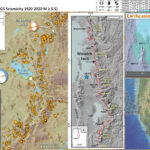
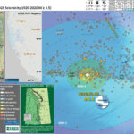
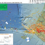
Well, it was a big mag 5 day today, two magnitude 5+ earthquakes in the western USA on faults related to the same plate boundary! Crazy, right? The same plate boundary, about 800 miles away from each other, and their coincident occurrence was in no way related to each other.
In the past 9 months it was also a big mag 5 MTJ year. There have been 3 mag 5+ earthquakes in the Mendocino triple junction (MTJ) region. The first one in June of 2019, at the time, appeared to be related to the Mendocino fault. The 9 March M 5.8 event was clearly associated with the right lateral Mendocino transform fault. The latest in this series of unrelated earthquakes is possibly associated with NW striking faults in the Gorda plate. I will discuss this below and include background about all the different faults in the region.

2019.06.23 M 5.6 Petrolia (USGS Page) (EarthJay Page)
2020.03.09 M 5.8 Mendocino fault (USGS Page) (EarthJay Page)
2020.03.18 M 5.2 Petrolia (USGS Page) (EarthJay Page – this one, lol)

I was on the phone with my friend, collaborator, and business partner Thomas Harvey Leroy (the man with 4 first names: Tom, Harvey, Lee, and Roy) yesterday afternoon. We were determining the best course of action after a tenant of ours moved out leaving PG&E with an unpaid ~$9000 bill and we could not turn the power back on until the bill was paid. His son walked up to him and asked if what he had just felt was an earthquake. Because Tom was pacing back and forth, he did not feel it (as Tom likes to say, “feel the pain.”). He wishes that he had felt it.
My social media feed was immediately dominated by posts about the earthquake in Humboldt County. I put together a quick map (see below). My good friend and collaborator Bob McPherson (a seismologist who ran the Humboldt Bay Seismic Network in the late 70s and 80s) sent me several text messages about the earthquake. we texted back and forth. I initially thought it might be Mendo fault and so did he.
Then the USGS moment tensor (earthquake mechanism) came in with an orientation similar to that of Gorda plate earthquakes further to the north. These earthquakes are typically on northeast striking (trending) left-lateral strike-slip faults (see more here about types of earthquakes). So, I stated that I thought it was like those, a left-lateral strike-slip fault earthquake. So I deleted my social media posts and updated the map to show it could be either left-lateral or right-lateral (the map below shows both options), but that we thought it was in the Gorda plate, not the Mendocino fault.

Then Bomac mentioned these northwest trends in seismicity that we noticed (as a group) about 5 years ago, seismicity trends (seismolineaments is what Tom calls them) that first appeared following the 1992 Cape Mendocino Earthquake.
We don’t yet have a full explanation for these trends in seismicity, but the orientation fits a stress field from north-south compression (from the northward motion of the Pacific plate relative to the Gorda plate). This north-south compression is also the explanation for the left-lateral strike-slip fault earthquakes in the Gorda plate (Silver, 1971).

How are these 3 M5+ MTJ events related?

Well, they are not directly related to each other (i.e. none of these earthquakes caused any of the other earthquakes). The exception is that the 2019 M 5.6 may have affected the stress in the crust leading to the March M 5.2, but this is unlikely. What is even less likely that the M 5.8 was caused by the June 5.6 or caused the march 5.2.
WHy?
Well, there are two kinds of earthquake triggering.

Dynamic Triggering – When seismic waves travel through the Earth, they change the stresses in the crust. IF the faults are “locked and loaded” (i.e. they are just about ready to slip in an earthquake), there may be an earthquake on the “receiver” fault. Generally, once the seismic waves are done travelling, this effect is over. Though, some suggest that this affect on the stress changes may last longer (but not much longer).
Static Triggering – When an earthquake fault slips, it deforms (changes the shape) of the crust surrounding that earthquake. These changes can cause increases and decreases in the stress on faults (either increasing or decreasing the chance for an earthquake). Just like for dynamic triggering, the fault needs to be about ready to slip. The effect on fault slip changes in “static coulomb stress” generally extend a distance of about 2-3 times the fault length of the “source” fault.

Below is a figure from Wells and Coppersmith (1994) that shows the empirical relations between surface rupture length (SRL, the length of the fault that ruptures to the ground surface) and magnitude. If one knows the SRL (horizontal axis), they can estimate the magnitude (vertical axis). The left plot shows the earthquake data. The right plot shows how their formulas “predict” these data.

(a) Regression of surface rupture length on magnitude (M). Regression line shown for all-slip-type relations. Short dashed line indicates 95% confidence interval. (b) Regression lines for strike-slip, reverse, and normal-slip relations. See Table 2 for regression coefficients. Length of regression lines shows the range of data for each relation.
* note, i corrected this caption by changing the word “relationships” to “relations.”

Using these empirical relations (which are crude and may not cover earthquakes as small as this M 5.8, but they are better than nothing), the “surface rupture length” of this M 5.8 might be about 5 km. So, changes in static coulomb stress from the M 5.8 extended, at most, about 16 km (or about 10 miles). Yesterday’s M 5.2. is about 72 km away, far too distant to be statically triggered by the 5.8.
The M 5.6 might have a rupture length crudely about 3 km might affect the region up to 9 km away. The M 5.2 is ~16 km from the M 5.6, so probably too far to be affected.
However, these earthquakes are related because they are all in the same region and are responding to the same tectonic forces.

Below is my interpretive poster for this earthquake

I plot the seismicity from the past month, with diameter representing magnitude (see legend). I include earthquake epicenters from 1919-2019 with magnitudes M ≥ 3.0 in one version.
I plot the USGS fault plane solutions (moment tensors in blue and focal mechanisms in orange), possibly in addition to some relevant historic earthquakes.
A review of the basic base map variations and data that I use for the interpretive posters can be found on the Earthquake Reports page.
Some basic fundamentals of earthquake geology and plate tectonics can be found on the Earthquake Plate Tectonic Fundamentals page.

I include some inset figures. Some of the same figures are located in different places on the larger scale map below.

In the upper left corner are a map of the tectonic plates and their boundary faults (Chaytor et al., 2006; Nelson et al., 2006). To the right is a and cross section cutting into the Earth from West (left) to East (right) that shows the downgoing (subducting) Gorda plate beneath the North America plate (Plafker, 1972).
In the upper right corner is a map of the MTJ area. The Great Salt Lake is the large light blue bleb in the upper right. We can see the mountains to the east of SLC, the Wasatch Range. The Earthquake Intensity uses the MMI scale (the colors), read more about this here. This map represents an estimate of ground shaking from the M 5.7 based on a statistical model using the results of tens of thousands of earthquakes.
In the lower left corner to the right of the legend is a plot showing how these USGS models “predict” the ground shaking intensity will be relative to distance from the earthquake. These models are represented by the broan and green lines. People can fill out an online form to enter their observations and these “Did You Feel It?” observations are converted into an intensity number and these are plotted as dots in this figure.
There are several sources of seismicity on this map, but i tried to make it easier to interpret using color choices. I recognize this poster does not satisfy Access and Functional Needs. I will work on that.

The three main earthquakes are plotted in pastel yellow and orange-yellow colors.
Earthquakes from the past 3 months are light green.
The earthquakes from the past century are faint gray.
The earthquakes located using a double differenced locating method are colored relative to depth.

Look at the westernmost NW trend in seismicity. How does the depth of the earthquakes change along that transect?
Yes! The earthquakes deepen to the southeast. These earthquakes are revealing to us the location (e.g. depth) of the Gorda plate as it dives deeper to the east.

Here is the map with 3 month’s (in green) and 1 century’s (in gray, mislabeled) seismicity plotted. I also include seismicity from a catalog with events relocated using the Double Differencing method.

I also outlined the two main northwest trends in seismicity with dashed white line polygons. The 18 March event is in the southern end of the western seismicity trend.
There is a nice northeast trend in seismicity that I also outlined. This is probably representative of one of the typical left-lateral Strike-slip Gorda plate earthquakes.

Other Report Pages

Some Relevant Discussion and Figures

Here is a map of the Cascadia subduction zone, modified from Nelson et al. (2006). The Juan de Fuca and Gorda plates subduct norteastwardly beneath the North America plate at rates ranging from 29- to 45-mm/yr. Sites where evidence of past earthquakes (paleoseismology) are denoted by white dots. Where there is also evidence for past CSZ tsunami, there are black dots. These paleoseismology sites are labeled (e.g. Humboldt Bay). Some submarine paleoseismology core sites are also shown as grey dots. The two main spreading ridges are not labeled, but the northern one is the Juan de Fuca ridge (where oceanic crust is formed for the Juan de Fuca plate) and the southern one is the Gorda rise (where the oceanic crust is formed for the Gorda plate).

Here is a version of the CSZ cross section alone (Plafker, 1972). This shows two parts of the earthquake cycle: the interseismic part (between earthquakes) and the coseismic part (during earthquakes). Regions that experience uplift during the interseismic period tend to experience subsidence during the coseismic period.

This poster includes seismicity from the past ~5 decades, for temblors M > 3.0. I also include the map and cross section as explained above. On the left is a map that shows the possible shaking intensity from a future CSZ earthquake.

More about the materials on this poster can be found on this page.

I have compiled some literature about the CSZ earthquake and tsunami. Here is a short list that might help us learn about what is contained within the core that I collected.

Hemphill-Haley, E., 1995. Diatom evidence for earthquake-induced subsidence and tsunami 300 yr ago in southern coastal Washington in GSA Bulletin, v. 107, p. 367-378.
Nelson, A.R., Shennan, I., and Long, A.J., 1996. Identifying coseismic subsidence in tidal-wetland stratigraphic sequences at the Cascadia subduction zone of western North America in Journal of Geophysical Research, v. 101, p. 6115-6135.
Atwater, B.F. and Hemphill-Haley, E., 1997. Recurrence Intervals for Great Earthquakes of the Past 3,500 Years at Northeastern Willapa Bay, Washington in U.S. Geological Survey Professional Paper 1576, Washington D.C., 119 pp.

This figure shows how a subduction zone deforms between (interseismic) and during (coseismic) earthquakes. We also can see how a subduction zone generates a tsunami. Atwater et al., 2005.

Here is an animation produced by the folks at Cal Tech following the 2004 Sumatra-Andaman subduction zone earthquake. I have several posts about that earthquake here and here. One may learn more about this animation, as well as download this animation here.

The Gorda and Juan de Fuca plates subduct beneath the North America plate to form the Cascadia subduction zone fault system. In 1992 there was a swarm of earthquakes with the magnitude Mw 7.2 Mainshock on 4/25. Initially this earthquake was interpreted to have been on the Cascadia subduction zone (CSZ). The moment tensor shows a compressional mechanism. However the two largest aftershocks on 4/26/1992 (Mw 6.5 and Mw 6.7), had strike-slip moment tensors. In my mind, these two aftershocks aligned on what may be the eastern extension of the Mendocino fault. However, looking at their locations, my mind was incorrect. These two earthquakes were not aftershocks, but were either left-lateral or right-lateral strike-slip Gorda plate earthquakes triggered by the M 7.1 thrust event.
These two quakes appear to be aligned with the two northwest trends in seismicity and the 18 March 2020 M 5.2. The orientation of the mechanisms are not as perfectly well aligned, but there are lots of reasons for this (perhaps the faults were formed in a slightly different orientation, but have rotated slightly).
There have been several series of intra-plate earthquakes in the Gorda plate. Two main shocks that I plot of this type of earthquake are the 1980 (Mw 7.2) and 2005 (Mw 7.2) earthquakes. I place orange lines approximately where the faults are that ruptured in 1980 and 2005. These are also plotted in the Rollins and Stein (2010) figure above. The Gorda plate is being deformed due to compression between the Pacific plate to the south and the Juan de Fuca plate to the north. Due to this north-south compression, the plate is deforming internally so that normal faults that formed at the spreading center (the Gorda Rise) are reactivated as left-lateral strike-slip faults. In 2014, there was another swarm of left-lateral earthquakes in the Gorda plate. I posted some material about the Gorda plate setting on this page.

Here is a link to the embedded video below, showing the week-long seismicity in April 1992.

This is the map used in the animation below. Earthquake epicenters are plotted (some with USGS moment tensors) for this region from 1917-2017 with M ≥ 6.5. I labeled the plates and shaded their general location in different colors.
I include some inset maps.

In the upper right corner is a map of the Cascadia subduction zone (Chaytor et al., 2004; Nelson et al., 2004).
In the upper left corner is a map from Rollins and Stein (2010). They plot epicenters and fault lines involved in earthquakes between 1976 and 2010.

Here is a map from Rollins and Stein, showing their interpretations of different historic earthquakes in the region. This was published in response to the Januray 2010 Gorda plate earthquake. The faults are from Chaytor et al. (2004).

Tectonic configuration of the Gorda deformation zone and locations and source models for 1976–2010 M ≥ 5.9 earthquakes. Letters designate chronological order of earthquakes (Table 1 and Appendix A). Plate motion vectors relative to the Pacific Plate (gray arrows in main diagram) are from Wilson [1989], with Cande and Kent’s [1995] timescale correction.

Here is a large scale map of the 1994 earthquake swarm. The mainshock epicenter is a black star and epicenters are denoted as white circles.

Here is a plot of focal mechanisms from the Dengler et al. (1995) paper in California Geology.

In this map below, I label a number of other significant earthquakes in this Mendocino triple junction region. Another historic right-lateral earthquake on the Mendocino fault system was in 1994. There was a series of earthquakes possibly along the easternmost section of the Mendocino fault system in late January 2015, here is my post about that earthquake series.

Here is a map from Chaytor et al. (2004) that shows some details of the faulting in the region. The moment tensor (at the moment i write this) shows a north-south striking fault with a reverse or thrust faulting mechanism. While this region of faulting is dominated by strike slip faults (and most all prior earthquake moment tensors showed strike slip earthquakes), when strike slip faults bend, they can create compression (transpression) and extension (transtension). This transpressive or transtentional deformation may produce thrust/reverse earthquakes or normal fault earthquakes, respectively. The transverse ranges north of Los Angeles are an example of uplift/transpression due to the bend in the San Andreas fault in that region.

A: Mapped faults and fault-related ridges within Gorda plate based on basement structure and surface morphology, overlain on bathymetric contours (gray lines—250 m interval). Approximate boundaries of three structural segments are also shown. Black arrows indicated approximate location of possible northwest- trending large-scale folds. B, C: uninterpreted and interpreted enlargements of center of plate showing location of interpreted second-generation strike-slip faults and features that they appear to offset. OSC—overlapping spreading center.

These are the models for tectonic deformation within the Gorda plate as presented by Jason Chaytor in 2004.

Models of brittle deformation for Gorda plate overlain on magnetic anomalies modified from Raff and Mason (1961). Models A–F were proposed prior to collection and analysis of full-plate multibeam data. Deformation model of Gulick et al. (2001) is included in model A. Model G represents modification of Stoddard’s (1987) flexural-slip model proposed in this paper.

Further North

If we move a little further north, we can take a look at the Blanco fault. This is a right-lateral strike-slip fault just like the Mendocino and San Andreas faults.
If we turn our head at an oblique angle, we may consider the San Andreas, the Mendocino, and the Blanco faults to be all part of the same transform fault.
Transform faults are often (or solely) defined as a strike-slip fault system that terminates at each end with a spreading ridge. These 3 systems link spreading ridges in the Gulf of California, through the Gorda Rise, to the Juan de Fuca ridge (and further).
The Blanco fault is as, or more active than the Mendocino fault. The excellent people in Oregon who are aware of their exposure to seismic and tsunami hazards from the Cascadia subduction zone are always interested when there are earthquake notifications.
Earthquakes on the Blanco fault are some of these events that people notice and ask about, “should I be concerned?” The answer is generally, “those earthquakes are too far away and too small to change the chance of the “Big One.” (remember the discussion about dynamic triggering above?)
There was a recent earthquake (2018) on the Blanco fault that brought the public to question this again. My report about that earthquake spent a little space addressing these fault length >> magnitude >> triggering issues.
As we know, the tectonics of the northeast Pacific is dominated by the Cascadia subduction zone, a convergent plate boundary, where the Explorer, Juan de Fuca, and Gorda oceanic plates dive eastward beneath the North America plate.
These oceanic plates are created (formed, though I love writing “created” in science writing) at oceanic spreading ridges/centers.
When oceanic spreading centers are offset laterally, a strike-slip fault forms called a transform fault. The Blanco transform fault is a right-lateral strike-slip fault (like the San Andreas fault). Thanks to Dr. Harold Tobin for pointing out why this is not a fracture zone.

This is the figure from Dziak et al. (2000) for us to evaluate. I include their long figure caption below.

(Top) Sea Beam bathymetric map of the Cascadia Depression, Blanco Ridge, and Gorda Depression, eastern Blanco Transform Fault Zone (BTFZ).Multibeam bathymetry was collected by the NOAA R/V’s Surveyor and Discoverer and the R/V Laney Chouest during 12 cruises in the 1980’s and 90’s. Bathymetry displayed using a 500 m grid interval. Numbers with arrows show look directions of three-dimensional diagrams in Figures 2 and 3. (Bottom) Structure map, interpreted from bathymetry, showing active faults and major geologic features of the region. Solid lines represent faults, dashed lines are fracture zones, and dotted lines show course of turbidite channels. When possible to estimate sense of motion on a fault, a filled circle shows the down-thrown side. Inset maps show location and generalized geologic structure of the BTFZ. Location of seismic reflection and gravity/magnetics profiles indicated by opposing brackets. D-D’ and E-E’ are the seismic reflection profiles shown in Figures 8a and 8b, and G-G’ is the gravity and magnetics profile shown in Figure 13. Submersible dive tracklines from sites 1 through 4 are highlighted in red. L1 and L2 are two lineations seen in three-dimensional bathymetry shown in Figures 2 and 3. Location of two Blanco Ridge slump scars indicated by half-rectangles, inferred direction of slump shown by arrow, and debris location (when identified) designated by an ‘S’. CD stands for Cascadia Depression, BR is Blanco Ridge, GD is Gorda Depression, and GR is Gorda Ridge. Numbers on north and south side of transform represent Juan de Fuca and Pacific plate crustal ages inferred from magnetic anomalies. Long-term plate motion rate between the Pacific and southern Juan de Fuca plates from Wilson (1989).

When there are quakes on the BF, people always wonder if the Cascadia megathrust is affected by this… “are we at greater risk because of those BF earthquakes?”
The main take away is that we are not at a greater risk because of these earthquakes.

Here is the map with a century’s seismicity plotted, for earthquakes of magnitude M ≥ 6.0 for the 29 Aug 2019 M 6.3 Blanco fault earthquake.

The poster includes earthquake information for earthquakes with M ≥ 6.0. I prepared this for a magnitude M 6.2 Blanco fault earthquake on 22 August 2018. I place fault mechanisms for all existing USGS mechanisms from the Blanco fracture zone and I include some examples from the rest of the region. These other mechanisms show how different areas have different tectonic regimes. Earthquakes within the Gorda plate are largely responding to being deformed in a tectonic die between the surrounding stronger plates (northeast striking (oriented) left-lateral strike-slip earthquakes). I include one earthquake along the Mendocino fracture zone, a right-lateral (dextral) strike-slip earthquake from 1994. I include one of the more memorable thrust earthquakes, the 1992 Cape Mendocino earthquake. I also include an extensional earthquake from central Oregon that may represent extension (basin and range?) in the northwestern region of the basin and range.

Cascadia subduction zone

General Overview

1700.09.26 M 9.0 Cascadia’s 315th Anniversary 2015.01.26
1700.09.26 M 9.0 Cascadia’s 316th Anniversary 2016.01.26 updated in 2017 and 2018
1992.04.25 M 7.1 Cape Mendocino 25 year remembrance
1992.04.25 M 7.1 Cape Mendocino 25 Year Remembrance Event Page
Earthquake Information about the CSZ 2015.10.08

Earthquake Reports

Explorer plate

Uncertain

2017.06.11 M 3.5 Gorda or NAP?

2016.07.21 M 4.7 Gorda or NAP? p-1
2016.07.21 M 4.7 Gorda or NAP? p-2

Social Media

References:

Basic & General References

Frisch, W., Meschede, M., Blakey, R., 2011. Plate Tectonics, Springer-Verlag, London, 213 pp.
Hayes, G., 2018, Slab2 – A Comprehensive Subduction Zone Geometry Model: U.S. Geological Survey data release, https://doi.org/10.5066/F7PV6JNV.
Holt, W. E., C. Kreemer, A. J. Haines, L. Estey, C. Meertens, G. Blewitt, and D. Lavallee (2005), Project helps constrain continental dynamics and seismic hazards, Eos Trans. AGU, 86(41), 383–387, , https://doi.org/10.1029/2005EO410002. /li>
Jessee, M.A.N., Hamburger, M. W., Allstadt, K., Wald, D. J., Robeson, S. M., Tanyas, H., et al. (2018). A global empirical model for near-real-time assessment of seismically induced landslides. Journal of Geophysical Research: Earth Surface, 123, 1835–1859. https://doi.org/10.1029/2017JF004494
Kreemer, C., J. Haines, W. Holt, G. Blewitt, and D. Lavallee (2000), On the determination of a global strain rate model, Geophys. J. Int., 52(10), 765–770.
Kreemer, C., W. E. Holt, and A. J. Haines (2003), An integrated global model of present-day plate motions and plate boundary deformation, Geophys. J. Int., 154(1), 8–34, , https://doi.org/10.1046/j.1365-246X.2003.01917.x.
Kreemer, C., G. Blewitt, E.C. Klein, 2014. A geodetic plate motion and Global Strain Rate Model in Geochemistry, Geophysics, Geosystems, v. 15, p. 3849-3889, https://doi.org/10.1002/2014GC005407.
Meyer, B., Saltus, R., Chulliat, a., 2017. EMAG2: Earth Magnetic Anomaly Grid (2-arc-minute resolution) Version 3. National Centers for Environmental Information, NOAA. Model. https://doi.org/10.7289/V5H70CVX
Müller, R.D., Sdrolias, M., Gaina, C. and Roest, W.R., 2008, Age spreading rates and spreading asymmetry of the world’s ocean crust in Geochemistry, Geophysics, Geosystems, 9, Q04006, https://doi.org/10.1029/2007GC001743
Pagani,M. , J. Garcia-Pelaez, R. Gee, K. Johnson, V. Poggi, R. Styron, G. Weatherill, M. Simionato, D. Viganò, L. Danciu, D. Monelli (2018). Global Earthquake Model (GEM) Seismic Hazard Map (version 2018.1 – December 2018), DOI: 10.13117/GEM-GLOBAL-SEISMIC-HAZARD-MAP-2018.1
Silva, V ., D Amo-Oduro, A Calderon, J Dabbeek, V Despotaki, L Martins, A Rao, M Simionato, D Viganò, C Yepes, A Acevedo, N Horspool, H Crowley, K Jaiswal, M Journeay, M Pittore, 2018. Global Earthquake Model (GEM) Seismic Risk Map (version 2018.1). https://doi.org/10.13117/GEM-GLOBAL-SEISMIC-RISK-MAP-2018.1
Zhu, J., Baise, L. G., Thompson, E. M., 2017, An Updated Geospatial Liquefaction Model for Global Application, Bulletin of the Seismological Society of America, 107, p 1365-1385, https://doi.org/0.1785/0120160198

Specific References

Atwater, B.F., Musumi-Rokkaku, S., Satake, K., Tsuju, Y., Eueda, K., and Yamaguchi, D.K., 2005. The Orphan Tsunami of 1700—Japanese Clues to a Parent Earthquake in North America, USGS Professional Paper 1707, USGS, Reston, VA, 144 pp.
Chaytor, J.D., Goldfinger, C., Dziak, R.P., and Fox, C.G., 2004. Active deformation of the Gorda plate: Constraining deformation models with new geophysical data: Geology v. 32, p. 353-356.
Dengler, L.A., Moley, K.M., McPherson, R.C., Pasyanos, M., Dewey, J.W., and Murray, M., 1995. The September 1, 1994 Mendocino Fault Earthquake, California Geology, Marc/April 1995, p. 43-53.
Geist, E.L. and Andrews D.J., 2000. Slip rates on San Francisco Bay area faults from anelastic deformation of the continental lithosphere, Journal of Geophysical Research, v. 105, no. B11, p. 25,543-25,552.
Irwin, W.P., 1990. Quaternary deformation, in Wallace, R.E. (ed.), 1990, The San Andreas Fault system, California: U.S. Geological Survey Professional Paper 1515, online at: http://pubs.usgs.gov/pp/1990/1515/
McCrory, P.A.,. Blair, J.L., Waldhauser, F., kand Oppenheimer, D.H., 2012. Juan de Fuca slab geometry and its relation to Wadati-Benioff zone seismicity in JGR, v. 117, B09306, doi:10.1029/2012JB009407.
McLaughlin, R.J., Sarna-Wojcicki, A.M., Wagner, D.L., Fleck, R.J., Langenheim, V.E., Jachens, R.C., Clahan, K., and Allen, J.R., 2012. Evolution of the Rodgers Creek–Maacama right-lateral fault system and associated basins east of the northward-migrating Mendocino Triple Junction, northern California in Geosphere, v. 8, no. 2., p. 342-373.
Nelson, A.R., Asquith, A.C., and Grant, W.C., 2004. Great Earthquakes and Tsunamis of the Past 2000 Years at the Salmon River Estuary, Central Oregon Coast, USA: Bulletin of the Seismological Society of America, Vol. 94, No. 4, pp. 1276–1292
Rollins, J.C. and Stein, R.S., 2010. Coulomb stress interactions among M ≥ 5.9 earthquakes in the Gorda deformation zone and on the Mendocino Fault Zone, Cascadia subduction zone, and northern San Andreas Fault: Journal of Geophysical Research, v. 115, B12306, doi:10.1029/2009JB007117, 2010.
Stoffer, P.W., 2006, Where’s the San Andreas Fault? A guidebook to tracing the fault on public lands in the San Francisco Bay region: U.S. Geological Survey General Interest Publication 16, 123 p., online at http://pubs.usgs.gov/gip/2006/16/
Wallace, Robert E., ed., 1990, The San Andreas fault system, California: U.S. Geological Survey Professional Paper 1515, 283 p. [http://pubs.usgs.gov/pp/1988/1434/].
Wells, D.L., and Coopersmith, K.J., 1994. New empirical relationships among magnitude, rupture length, rupture width, rupture area, and surface displacement in BSSA, v. 84, no. 4, p. 974-1002

Return to the Earthquake Reports page.

Sorted by Magnitude
Sorted by Year
Sorted By Region

Earthquake Report: Salt Lake City

Posted on March 18, 2020 by Jay Patton

As I was waking up this morning, I rolled over to check my social media feed and moments earlier there was a good sized shaker in Salt Lake City, Utah. I immediately thought of my good friend Jennifer G. who lives there with her children. I immediately started looking into this earthquake.
https://earthquake.usgs.gov/earthquakes/eventpage/uu60363602/executive
The second thing I thought of was Chris DuRoss, a USGS geologist I first met when he was presenting his research of the record of prehistoric earthquakes along the Wasatch fault at the Seismological Society of America (SSA) meeting that was being held in SLC that year. Gosh, that was in 2013. My, how time passes. Dr. DuRoss now works for the USGS and continues to research the seismic hazards of the intermountain west and beyond from his office in Golden, Colorado.
The third thing I thought of was all the buildings in the SLC area that are not designed to withstand the shaking from the earthquakes that we expect will occur on that fault system. About 85% of the population of the state of Utah lives within 15 miles of the Wasatch fault. This is sobering.
I quickly put together a poster for this earthquake to help people learn a little more. I have a second earthquake to interpret tonight, so I will update this report later with more background on the Wasatch fault tectonics and seismic hazard.
There is also a great resource from the University of Utah, an event page for this earthquake sequence.

Tectonic Background

The west coast of the United States and Mexico is dominated by the plate boundary between the Pacific and North America plates. Many are familiar with the big players in this system:

The right-lateral transform fault zone called the San Andreas fault (SAF) where the North America plate on the east moves south relative to the Pacific plate. They are both moving north-ish, but the Pacific plate is moving “North” faster than the North America plate.
The convergent plate boundary called the Cascadia subduction zone (CSZ) where the Gorda, Juan de Fuca, and Explorer plates are diving beneath the North America plate, forming a megathrust subduction fault system.

There are many other faults that are also part of this plate boundary system. The San Andreas fault zone “proper” accommodates about 85% of the relative plate motion. The rest of the relative plate motion (15%) is accounted for by slip on other strike-slip fault systems.
There are “sibling” faults to the SAF near the SAF (like the Hayward fault in the San Francisco Bay Area) and further away (like the Eastern California shear zone, the Owens Valley fault, and the Walker Lane fault systems).
Just like Dr. Steve Wesnousky showed us, the crust in the Walker Lane is moving around like a layer of solid wax floating around on a tray of melted wax. So, there are faults in lots of different kinds of directions, and different kinds of faults too.
The easternmost right-lateral strike slip fault is the Wasatch fault.
East of Sierra Nevada. in Nevada and western Utah, there is lots of East-West oriented extension (i.e. the Basin and Range) where the crust in western Nevada is moving west compared to the crust in Salt Lake City, Utah.
The Wasatch is also one of these extensional faults we call Normal faults.
In Salt Lake City, the Wasatch fault is oriented roughly north-south and is generally located on the eastern side of the valley, near the base of the mountains. The Crust on the western side of the fault is moving west relative to the mountains.
The fault then dips down towards the west. Because the motion is east-west, and the fault dips at an angle, the valley goes down over time relative to the mountains (thus forming the valley).
Today’s earthquake happened in the middle of the valley, where the Wasatch fault is deep beneath. The earthquake was a “normal” fault earthquake with east-west extension. So, the earthquake and aftershocks are on a fault related to the Wasatch (or we are wrong about the precise location of the fault, the earthquake, or both).
The USGS has an earthquake forecast product where the scientists at the Earthquake Center use a statistical model to estimate the possibility of earthquakes of different magnitude ranges may occur in the future over ranges of time periods after the main earthquake.
Don’t run outside during an earthquake.

Below is my interpretive poster for this earthquake

I plot the seismicity from the past month, with diameter representing magnitude (see legend). I include earthquake epicenters from 1919-2019 with magnitudes M ≥ 3.0 in one version.
I plot the USGS fault plane solutions (moment tensors in blue and focal mechanisms in orange), possibly in addition to some relevant historic earthquakes.
A review of the basic base map variations and data that I use for the interpretive posters can be found on the Earthquake Reports page.
Some basic fundamentals of earthquake geology and plate tectonics can be found on the Earthquake Plate Tectonic Fundamentals page.

I include some inset figures. Some of the same figures are located in different places on the larger scale map below.

In the lower right corner is a map of the western USA with USGS seismicity from the past century for earthquakes M 5.5+. Note all the north-south oriented lines in Nevada and Utah. These are formed by all the normal faults from the east-west extension in the basin and range.
In the upper right corner is a map of the Salt Lake City (SLC) area. The Great Salt Lake is the large light blue bleb in the upper right. We can see the mountains to the east of SLC, the Wasatch Range. The Earthquake Intensity uses the MMI scale (the colors), read more about this here. This map represents an estimate of ground shaking from the M 5.7 based on a statistical model using the results of tens of thousands of earthquakes.
In the upper left corner is a plot showing how these USGS models “predict” the ground shaking intensity will be relative to distance from the earthquake. These models are represented by the broan and green lines. People can fill out an online form to enter their observations and these “Did You Feel It?” observations are converted into an intensity number and these are plotted as dots in this figure.
In the left-center is a map from DuRoss et al. (2016) that shows the Wasatch fault along the base of the Wasatch Range. Note that the fault is subdivided into different segments. We think that sometimes these different segments may rupture at different times and sometimes some of them may rupture at the same time.I placed a blue star in the location of today’s earthquake (projected onto the surface).

Here is the map with 1 year’s and 1 century’s seismicity plotted.

Two great resources for information about the tectonics of Utah are here:

Emily Kleber fromt he Utah Geological Survey put together this excellent overview.
Here is a Handbook for earthquakes in Utah. This is a pdf and can be printed out for the use in lesson plans for a variety of age groups. I particularly like the artwork on the cover.

Here is a clearinghouse of photos of damage from the earthquake (h/t to Nick Graehl, my coworker, for pointing this out).

Other Report Pages

Some Relevant Discussion and Figures

Here is the map from DuRoss et al. (2016).
The main fault is in red. There are additional faults, like the white lines west of Salt Lake City. These are traces of the West Valley fault zone (WVFZ). Note the next mountain range to the west (left) and that there is another north-south series of faults drawn at the base of those mountains too. This is the Oquirrh Great Salt Lake fault zone, a series of west dipping faults (just like the Wasatch fault)
The Wasatch fault is very long and notice how it is not continuous. One of the important things that we may want to know is if these all slip at the same time during an earthquake, or only some of them slip, or just one of them. This is one of the largest sources of uncertainty when it comes to estimating the seismic hazard of a region.
The authors (and others before them) subdivided the segments and these segments are labeled on this map.

Central segments of the WFZ (red), which have evidence of repeated Holocene surface-faulting earthquakes. Circles indicate sites with data that we reanalyzed using OxCal (abbreviations shown in Table 2); triangles indicate sites where data or documentation was inadequate for reanalysis (HC, Hobble Creek; PP, Pole Patch; WC, Water Canyon; WH, Woodland Hills). Other Quaternary faults in northern Utah (white lines) include the ECFZ, East Cache fault zone; OGSLFZ, Oquirrh Great Salt Lake fault zone; ULFF, Utah Lake faults and folds; WVFZ, West Valley fault zone. Fault traces are from Black et al. [2003]. Horizontal bars mark primary segment boundaries. Inset map shows the trace of the WFZ in northern Utah and southern Idaho.

This is a figure that shows what we think may be the way that these fault segments link (or not) through time (DuRoss et la., 2016).
The fault line map is on top (note how North is not always “up.”). The bottom chart aligns with the fault segments (along the north south distance represented by the red dashed and dotted line in the map).
The vertical axis is time in thousands of years ago (1950 is on the bottom and 7 thousand years ago is on top). Each blue bar represents the time that an earthquake may haven happened in the past and how those earthquakes may match the earthquake history of an adjacent segment.
If the blue bar on one segment matches the age range for an adjacent fault, that earthquake may have involved both segments. However due to the limitation with radiocarbon, we can never really know this.

Late Holocene surface-faulting earthquakes identified at trench sites along the central WFZ. Circles with labels indicate sites with data that were reanalyzed using OxCal, and unlabeled white triangles indicate sites where data or documentation was inadequate for reanalysis. Distance is measured along simplified fault trace (dash dotted line) shown in top panel. Individual earthquake-timing probability density functions (PDFs) and mean times are derived from OxCal models for the paleoseismic sites; number in brackets is event number, where one is the youngest.

Here is a cross section, showing us what we think may be how the faults extend beneath the ground surface. Drt, DuRoss tweeted this today.
The Wasatch fault begins on the right, at the base of the Wasatch Mountains and dips to the west (to the left) beneath Salt Lake City.
There are additional (antithetic) faults dipping to the east and these are called the West Valley fault zone. They are also normal faults formed from extension.
These faults are plotted in white in the above map.
The earthquake location is also plotted using two different information sources. According to Dr. RuRoss, these earthquakes may have happened on a previously unknown fault.

Earthquake Triggered Landslides

FOS = Resisting Force / Driving Force

When FOS > 1, the slope is stable and when FOS < 1, the slope fails and we get a landslide. The illustration below shows these relations. Note how the slope angle α can take part in this ratio (the steeper the slope, the greater impact of the mass of the slope can contribute to driving forces). The real world is more complicated than the simplified illustration below.

Landslide ground shaking can change the Factor of Safety in several ways that might increase the driving force or decrease the resisting force. Keefer (1984) studied a global data set of earthquake triggered landslides and found that larger earthquakes trigger larger and more numerous landslides across a larger area than do smaller earthquakes. Earthquakes can cause landslides because the seismic waves can cause the driving force to increase (the earthquake motions can “push” the land downwards), leading to a landslide. In addition, ground shaking can change the strength of these earth materials (a form of resisting force) with a process called liquefaction.
Sediment or soil strength is based upon the ability for sediment particles to push against each other without moving. This is a combination of friction and the forces exerted between these particles. This is loosely what we call the “angle of internal friction.” Liquefaction is a process by which pore pressure increases cause water to push out against the sediment particles so that they are no longer touching.
An analogy that some may be familiar with relates to a visit to the beach. When one is walking on the wet sand near the shoreline, the sand may hold the weight of our body generally pretty well. However, if we stop and vibrate our feet back and forth, this causes pore pressure to increase and we sink into the sand as the sand liquefies. Or, at least our feet sink into the sand.
Below is a diagram showing how an increase in pore pressure can push against the sediment particles so that they are not touching any more. This allows the particles to move around and this is why our feet sink in the sand in the analogy above. This is also what changes the strength of earth materials such that a landslide can be triggered.

Below is a diagram based upon a publication designed to educate the public about landslides and the processes that trigger them (USGS, 2004). Additional background information about landslide types can be found in Highland et al. (2008). There was a variety of landslide types that can be observed surrounding the earthquake region. So, this illustration can help people when they observing the landscape response to the earthquake whether they are using aerial imagery, photos in newspaper or website articles, or videos on social media. Will you be able to locate a landslide scarp or the toe of a landslide? This figure shows a rotational landslide, one where the land rotates along a curvilinear failure surface.

Here is a map that I put together using the data available from the USGS Earthquake Event pages. More about these models can be found here.
The map shows liquefaction susceptibility from the M 5.7 earthquake.
These models use empirical relations (earthquake data) between earthquake size, earthquake distance, and material properties of the Earth.
The largest assumption is that for the Earth materials. This model uses a global model for the seismic velocity in the upper 30 meters (i.e. the Vs30). This global model basically takes the topographic slope of the ground surface and converts that to Vs30. So, the model is basically based on a slope map. This is imperfect, but works moderately well at a global scale. A model based on real Earth material data would be much much better.