Earthquake Report: Cotobato Trench, Philippines

Posted on April 30, 2017 by Jay Patton

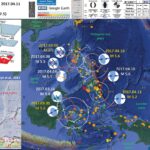
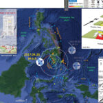
Earlier in April (2017) there was some activity in 4 different regions of the Philippines. Based upon the low magnitudes and large epicentral distances, these earthquakes were most unlikely to be directly related to each other.

A couple days ago, there was an earthquake along-dip from one of these earlier swarms. Here is the USGS web page for this M 6.9 earthquake.

There does not appear to have been an observed tsunami based upon a quick look at gages posted to this IOC site (though the closest 2 gages seem to have intermittent records).

The along dip seismicity earlier this month was along the Philippine trench subduction zone fault. The M 6.9 earthquake appears to be related to subduction along the Cotobato trench.

These earthquakes are ~300 km from each other. Also, the Philippine trench swarm appears to possibly have reduced stress on the Cotobato trench, but I might be wrong. Regardless, it is probably a coincidence that these earthquakes are along dip to each other.

Another coincidence is another earthquake along-dip to these earthquakes, a deep M 7.3 earthquake in the Celebes Sea in January 2017. Here is my earthquake report for this earthquake.

This is my Earthquake Report for these earlier earthquakes.
Here is another blog about the earthquakes near Manila (including the M 5.9): Stephen Hicks
UPDATE: here is the Berkeley Seismo Blog page for these earthquakes.
Here is another blog about the earthquakes near Manila (including the M 5.9): Stephen Hicks
Here is the Berkeley Seismo Blog page for these earthquakes.

Below is my interpretive poster for this earthquake.

I plot the seismicity from the past month, with color representing depth and diameter representing magnitude (see legend).

I placed a moment tensor / focal mechanism legend on the poster. There is more material from the USGS web sites about moment tensors and focal mechanisms (the beach ball symbols). Both moment tensors and focal mechanisms are solutions to seismologic data that reveal two possible interpretations for fault orientation and sense of motion. One must use other information, like the regional tectonics, to interpret which of the two possibilities is more likely.
I also include the shaking intensity contours on the map. These use the Modified Mercalli Intensity Scale (MMI; see the legend on the map). This is based upon a computer model estimate of ground motions, different from the “Did You Feel It?” estimate of ground motions that is actually based on real observations. The MMI is a qualitative measure of shaking intensity. More on the MMI scale can be found here and here. This is based upon a computer model estimate of ground motions, different from the “Did You Feel It?” estimate of ground motions that is actually based on real observations.
I include the slab contours plotted (Hayes et al., 2012), which are contours that represent the depth to the subduction zone fault. These are mostly based upon seismicity. The depths of the earthquakes have considerable error and do not all occur along the subduction zone faults, so these slab contours are simply the best estimate for the location of the fault.

I include some inset figures in the poster.

In the upper right corner is a figure from Hall (2011). This shows the plate tectonic configuration in the equatorial Pacific with a low angle oblique perspective. Note how the upper panel shows a west dipping slab on the east side of the Philippines. Note the contrast in the center panel (Halmahera), where the eastern fault is dipping to the east (westward vergent) and the western fault is dipping to the west (eastward vergent). This region near Halmahera forms the Molucca Strait, one of the most tectonically active areas in this region.
In the upper left corner is a map showing the regional tectonics from Smoczyck et al. (2013). Earthquakes are plotted with color representing depth and diameter representing magnitude (see legend). The Philippine trench is an eastward vergent (dipping to the west) subduction zone on the east side of the Philippines. The Manila trench and Cotoban trench are westward vergent (dipping to the east) subduction zone faults on the western side of the Philippines. Below the map I include the cross section showing earthquake hypocenters from this Smoczyck et al. (2013) publication (see legend). I placed a blue star in the general location of the M 6.9 Cotobato trench earthquake and a transparent blue star in the region of the M 5.6 and M 5.7 Philippine trench earthquakes on both the map and the cross section.
In the lower right corner I include a map showing the tectonics from the Molucca Sea (Waltham et al., 2008). I highlit the Cotobato trench in red. This map overlaps with the southern 75% of the Hall (2011) low-angle oblique figure above. This is a really interesting configuration. To the north, the subduction zones oppose each other (eastward vergent on the east and westward vergent on the west). Along the latitude of the Molucca Strait, the uppermost thrust faults have a similar opposing vergence. In contrast, the molucca sea plate is below these more shallow thrusts and forms opposing subduction zones with different polarity (eastward vergent on the east and westward vergent on the west).

Here is my poster for the earthquakes earlier this month.

This is the low-angle oblique view of the region (Hall, 2011).

3D cartoon of plate boundaries in the Molucca Sea region modified from Hall et al. (1995). Although seismicity identifies a number of plates there are no continuous boundaries, and the Cotobato, North Sulawesi and Philippine Trenches are all intraplate features. The apparent distinction between different crust types, such as Australian continental crust and oceanic crust of the Philippine and Molucca Sea, is partly a boundary inactive since the Early Miocene (east Sulawesi) and partly a younger but now probably inactive boundary of the Sorong Fault. The upper crust of this entire region is deforming in a much more continuous way than suggested by this cartoon.

This is the tectonic map from Waltham et al. (2008)

(A) Location and major tectonic features of the Molucca Sea region. Small, black-filled triangles are modern volcanoes. Bathymetric contours are at 200, 2000, 4000, and 6000 m. Large barbed lines are subduction zones, and small barbed lines are thrusts. (B) Cross section across the Halmahera and Sangihe Arcs on section line B. Thrusts on each side of the Molucca Sea are directed outward toward the adjacent arcs, although the subducting Molucca Sea plate dips east beneath Halmahera and west below the Sangihe Arc. (C) Inset is the restored cross section of the Miocene–Pliocene Weda Bay Basin of SW Halmahera on section line C, fl attened to the Pliocene unconformity, showing estimated thickness of the section.

This is smaller scale tectonic map of the region (Zahirovic et al., 2014).

Regional tectonic setting with plate boundaries (MORs/transforms = black, subduction zones = teethed red) from Bird (2003) and ophiolite belts representing sutures modified from Hutchison (1975) and Baldwin et al. (2012). West Sulawesi basalts are from Polvé et al. (1997), fracture zones are from Matthews et al. (2011) and basin outlines are from Hearn et al. (2003). ANI – Andaman and Nicobar Islands, BD– Billiton Depression, Ba – Bangka Island, BI – Belitung (Billiton) Island, BiS – Bismarck Sea, BP – Benham Plateau, CaR – Caroline Ridge, CS – Celebes Sea, DG– Dangerous Grounds, EauR – Eauripik Ridge, FIN – Finisterre Terrane, GoT – Gulf of Thailand, GR– Gagua Ridge, HAL– Halmahera, HBa – Huatung Basin, KB–Ketungau Basin, KP – Khorat Platform, KT – Kiilsgaard Trough, LS – Luconia Shoals, MacB – Macclesfield Bank, ManTr – Manus Trench, MaTr – Mariana Trench, MB– Melawi Basin, MDB– Minami Daito Basin, MG– Mangkalihat, MIN – Mindoro, MN– Mawgyi Nappe, MoS – Molucca Sea, MS– Makassar Straits, MTr – Mussau Trench, NGTr – New Guinea Trench, NI – Natuna Islands, ODR– Oki Daito Ridge, OJP –Ontong Java Plateau, OSF – Owen Stanley Fault, PAL – Palawan, PhF – Philippine Fault, PT – Paternoster Platform, PTr – Palau Trench, PVB – Parece Vela Basin, RB – Reed Bank, RMF– Ramu-Markham Fault, RRF – Red River fault, SEM– Semitau, ShB – Shikoku Basin, Sol. Sea – Solomon Sea, SPK – Sepik, SPT – abah–Palawan Trough, STr – Sorol Trough, Sul – Sulawesi, SuS – Sulu Sea, TPAA– Torricelli–Prince Alexander Arc, WB–West Burma, WCT–W Caroline Trough, YTr –Yap Trough.

This is a map and series of cross sections showing subducting plates in blue (Zahirovic et al., 2014). The cross sections are based upon seismic wave tomography, which is similar to CT scans (Computed Tomography of X-Rays). These two processes use the same general methods to investigate the 3-dimensional views of internal structures (bodies vs. the Earth). More can be found in their paper, but basically, the blue regions represent areas that have higher seismic velocity. Oceanic lithosphere has higher seismic velocities than the surrounding mantle. So, the subducting oceanic slabs show up as blue. The corss section G-G’ is at about the same latitude as the M 5.6-7 and M 6.9 earthquakes. Note that the Philippine sea plate subducting at the Philippine trench (dipping to the west/left) is evident, while the slab associated with the Cotobato trench does not appear visible. Compare this with the seismicity cross section from Smoczyck et al. (2013), where the Cotobato trench seismicity is much more shallow than the Philippine trench.

Vertical sections from MIT-P (Li et al., 2008) and GyPSuM-S (Simmons et al., 2009) seismic tomography models along profiles A to E (magenta lines). The first-order differences between the P- and S-wave models is that the amplitude of the positive seismic velocity anomalies significantly diminishes away from continental coverage (e.g., dashed lines in profiles A and B). A depth slice at 746 km from MIT-P isprovided for reference with super-imposed present-day coastlines and plate boundaries. Interpreted slab sources are labeled: GI-BA= Greater India–Neo-Tethyan back-arc slab, M/N-T – Meso- and Neo-Tethyan slabs, W-S –Woyla–Sunda slabs, S – Sunda slab, PSCS – proto-South China Sea slab, PAC – Pacific slab, PMOL– proto-Molucca slab, PSOL – proto-Solomon slab, CS – Caroline slab, PSP – Philippine Sea Plate slab, S-C = Sulu–Celebes slabs.

However, here is a figure that shows isosurfaces from their tomography models (Zahirovic et al., 2014). This shows what may be slabs related to the Cotobato trench (western part of G-G’ cross section). These slabs show up better on the lower figure.

3-D visualization of +0.2% seismic velocity anomaly isosurfaces in MIT-P (top) and +0.9% seismic velocity perturbation in GyPSuM-S (bottom) models. Profiles A to G represent the vertical profiles (see Fig. 10) that capture the convergence and subduction histories of the region since the Cretaceous. Present-day coastlines are translucent grey shades, and present-day plate boundaries are translucent black lines. Slab volumes are colored by their depth, while the light blue color represents the interior surface of these slabs. PSCS – proto-South China Sea slab.

In January of this year (2017), there was an M 7.3 earthquake in the Celebes Sea south of the Philippines. Below is my interpretive map for that earthquake. I also present the same poster with 1917-2017 seismicity for earthquakes M ≥ 6.5. Here is my earthquake report for this M 7.3 earthquake. I include more background information for the Molucca Strait region on this page.

References:

Bock et al., 2003. Crustal motion in Indonesia from Global Positioning System measurements in JGR, v./ 108, no. B8, 2367, doi:10.1029/2001JB000324
Hall, R., 2011. Australia–SE Asia collision: plate tectonics and crustal flow in Hall, R., Cottam, M. A. &Wilson, M. E. J. (eds) The SE Asian Gateway: History and Tectonics of the Australia–Asia Collision. Geological Society, London, Special Publications, 355, 75–109.
Hayes, G.P., Wald, D.J., and Johnson, R.L., 2012. Slab1.0: A three-dimensional model of global subduction zone geometries in, J. Geophys. Res., 117, B01302, doi:10.1029/2011JB008524
McCaffrey, R., Silver, E.A., and Raitt, R.W., 1980. Crustal Structure of the Molucca Sea Collision Zone, Indonesia in The Tectonic and Geologic Evolution of Southeast Asian Seas and Islands-Geophysical Monograph 23, p. 161-177.
Nelson, A.R., Personius, S.F., Rimando, R.E., Punongbayan, R.S., Tungol, N, Mirabueno, H., and Rasdas, A., 2000. Multiple Large Earthquakes in the Past 1500 Years on a Fault in Metropolitan Manila, the Philippines in BSSA vol. 90, p. 73-85.
Noda, A., 2013. Strike-Slip Basin – Its Configuration and Sedimentary Facies in Mechanism of Sedimentary Basin Formation – Multidisciplinary Approach on Active Plate Margins http://www.intechopen.com/books/mechanism-of-sedimentarybasin-formation-multidisciplinary-approach-on-active-plate-margins http://dx.doi.org/10.5772/56593
Smoczyk, G.M., Hayes, G.P., Hamburger, M.W., Benz, H.M., Villaseñor, Antonio, and Furlong, K.P., 2013. Seismicity of the Earth 1900–2012 Philippine Sea plate and vicinity: U.S. Geological Survey Open-File Report 2010–1083-M, 1 sheet, scale 1:10,000,000.
Waltham et al., 2008. Basin formation by volcanic arc loading in GSA Special Papers 2008, v. 436, p. 11-26.
Zahirovic et al., 2014. The Cretaceous and Cenozoic tectonic evolution of Southeast Asia in Solid Earth, v. 5, p. 227-273, doi:10.5194/se-5-227-2014.

Earthquake Report: Chile Update #2

Posted on April 28, 2017 by Jay Patton

Today the swarm has reminded us to stay vigilant. This region of the Chile subduction zone is pretty active and adjacent to the most active part of the Chile subduction zone. Today there was a series of earthquakes with a maximum magnitude of M 5.9. Here is the USGS webpage for this M 5.9 earthquake.

I have prepared several other reports for the recent seismicity here. More background information about the subduction zone history can be found there.
2017.04.23 M 5.9
2017.04.24 M 6.9
2017.04.24 M 6.9 Update #1

The current sequence is just to the south of the 1971 M 7.0 earthquake and has a similar along-strike distance. This may be all that we will see, but there is a small chance this will lead to an earthquake with a larger magnitude. I suspect this chance is not very high (low likelihood). If we consider the 1985 earthquake as an analog, there were only a few earthquakes prior to the mainshock. The 2017 swarm has had many earthquakes to date. I suspect that the M 6.9 is the mainshock for this series. Also, consider that the 1985 region overlaps slightly with the 2010 earthquake. While this region was an area of low slip in 2010, there might be a reason for this (e.g. the Juan Fernandez Ridge, JFR). The JFR may act as an asperity. Asperities have 2 main definitions: (1) region of largest slip during an earthquake (2) region of a fault across which strain is accumulated due to the material properties of the fault and crust. I use the second definition. Smooth subduction zone faults may be responsible for large magnitude earthquakes and rough subduction zone faults (with asperities like the JFR) may be responsible for smaller, more frequent, earthquakes. If we look at the Métois et al. (2016) figure below, this region of the subduction zone has a high rate of seismicity. If this seismicity is the result of a rough fault, it seems that this part of the megathrust may not store as much strain as other parts of the subduction zone. However, this part of the fault has slipped during Great earthquakes (M > 8.0) in the past. So, it is difficult to say. While I might be wrong, given what we know about this subduction zone, it seems like this swarm is not going to result in a Great earthquake this time. Others disagree with me and that is great! I am only looking at the seismicity from the past and others are actively testing the cycling of seismic strain (and coulomb stress) in this region.

von Huene et al. (1997), Tectonic control of the subducting Juan Fernandez Ridge on the Andean margin near Valparaiso, Chile
and Rodrigo and Lara (2014) Plate tectonics and the origin of the Juan Fernández Ridge: analysis of bathymetry and magnetic patterns.

I include the moment tensors from each of the Great Earthquakes, as well as the 2017 M 5.9, 6.9, and 5.9 earthquakes.

In the interpretive poster below

I outline the 1985 aftershock region in black dashed lines
I outline the 2010 aftershock region in blue dashed lines
I outline the 2015 aftershock region in white dashed lines
I outline the 2017 aftershock region in red dashed lines

Below is my interpretive poster for this earthquake. Click on the map to enlarge.

I placed a moment tensor / focal mechanism legend on the poster. There is more material from the USGS web sites about moment tensors and focal mechanisms (the beach ball symbols). Both moment tensors and focal mechanisms are solutions to seismologic data that reveal two possible interpretations for fault orientation and sense of motion. One must use other information, like the regional tectonics, to interpret which of the two possibilities is more likely.
I also include the shaking intensity contours on the map. These use the Modified Mercalli Intensity Scale (MMI; see the legend on the map). This is based upon a computer model estimate of ground motions, different from the “Did You Feel It?” estimate of ground motions that is actually based on real observations. The MMI is a qualitative measure of shaking intensity. More on the MMI scale can be found here and here. This is based upon a computer model estimate of ground motions, different from the “Did You Feel It?” estimate of ground motions that is actually based on real observations.
I include the slab contours plotted (Hayes et al., 2012), which are contours that represent the depth to the subduction zone fault. These are mostly based upon seismicity. The depths of the earthquakes have considerable error and do not all occur along the subduction zone faults, so these slab contours are simply the best estimate for the location of the fault.

I include one inset figure in the poster.

In the lower right corner I present the space-time diagram from Métois et al. (2016). They plot seismicity vs. depth on the right. I placed a green bar with the approximate latitudinal range of the 2017 sequence.
In the lower left corner I present the figure from Métois et al. (2016) that shows their estimates of seismic coupling (the proportion of the fault that is “locked” and accumulating strain). Regions of low coupling do not accumulate strain, do not resist earthquake rupture, and do not contribute to the release of energy during earthquakes.
I place a green bar as for the space time figure on the right. Note the high rate of seismicity in this region. Also, note that the region of the fault that is participating in this 2017 sequence is a region of lower coupling between the 2015 and 2010 patches. One problem is that the 2015 patch did not release much strain in the higher coupled area (though this area has more earthquakes, so that might release strain, limiting the possibility of future larger earthquakes.
In the upper right corner, I plot seismicity for the past 2.5 months along with the 30 day seismicity surrounding the 1985 earthquake. I also outline the 1985 and 2017 sequences.

Here is the space time figure from Métois et al. (2016).

Left estimated extent of large historical or instrumental ruptures along the Chilean margin adapted from ME´ TOIS et al. (2012). Gray stars mark major intra-slab events. The recent Mw[8 earthquakes are indicated in red. Gray shaded areas correspond to LCZs defined in Fig. 3. Right seismicity recorded by the Centro Sismologico Nacional (CSN) during interseismic period, color-coded depending on the event’s depth. Three zones have been defined to avoid including aftershocks and preshocks associated with major events: (1) in North Chile, we plot the seismicity from 2008 to january 2014, i.e., between the Tocopilla and Iquique earthquakes; (2) in Central Chile, we plot the seismicity on the entire 2000–2014 period; (3) in South-Central Chile, we selected events that occurred between 2000 and 2010, i.e., before the Maule earthquake.

Here is the seismic coupling figure from Métois et al. (2016).

a Histogram depicts the rate of Mw[3 earthquakes registered by the CSN catalog during the interseismic period defined for each zone (see Fig. 2) on the subduction interface, on 0.2 of latitude sliding windows. Stars are swarm-like sequences detected by HOLTKAMP et al. (2011) depending on their occurrence date. Swarms located in the Iquique LCZ and Camarones segment are from RUIZ et al. (2014). Empty squares are significant intraplate earthquakes. b Red curve variations of the average coupling coefficient on the first 60 km of depth calculated on 0.2 of latitude sliding windows for our best model including an Andean sliver motion. Dashed pink curves are alternative models with different smoothing options that fit the data with nRMS better than 2 (see supplementary figure 6): the pink shaded envelope around our best model stands for the variability of the coupling along strike. Green curves coseismic distribution for Maule (VIGNY et al. 2011), Iquique (LAY et al. 2014) and Illapel earthquakes (RUIZ et al. 2016). Gray shaded areas stand for the identified low coupling zones (LCZs). LCZs and high coupling segments are named on the left. The apparent decrease in the average coupling North of 30S is considered as an artifact of the Andean sliver motion (see Sect. 5.2). c Best coupling distribution obtained inverting for Andean sliver motion and coupling amount simultaneously. The rupture zones for the three major earthquakes are indicated as green ellipses. White shaded areas are zones where we lack resolution

Here is a figure from Conteras-Reyes and Carrizo, 2011 that shows how the structure of the Nazca plate may exert heterogeneous forces along the subduction zone fault.

(upper) Structure and interpretation of the (A) Nazca Ridge, (B) easternmost portion of the Juan Fernández Ridge, and (C) Mocha FZ based on the 2D seismic velocity model of Hampel et al. (2004), Kopp et al. (2004), and Contreras-Reyes et al. (2008), respectively. Map locations of seismic profiles are shown in Fig. 1A. (below) Direct comparison of these HOF’s structure with typical Nazca oceanic crust (6.5km thick). The anomalous normal stress n (buoyancy force) depends on the thickness of the corresponding anomalous crustal thickness (Hc) and on thickness of the underplated magmatic material beneath the crust and/or thickness of the serpentinized mantle (Hm). n also depends on the mantle–crust density contrast (mc = 530 kg/m3), “normal” mantle–serpentinized mantle density contrast (m= 230 kg/m3) and “normal” crust-altered crust density contrast (c = 50 kg/m3). See further details in Table 1. Density values are taken from the density model of Tassara et al. (2006).

Some background about the heterogeneous megathrust in this region

Here is the first of two figures from Moreno et al., 2010. Note that the M 6.9 is close in space to the 1985 earthquake. Also note the along strike heterogeneous seismogenic coupling. I include the figure caption below in blockquote.

Tectonic setting of the study area, data, observations and results. a, Shaded relief map of the Andean subduction zone in South- Central Chile. Earthquake segmentation along the margin is indicated by ellipses that enclose the approximate rupture areas of historic earthquakes (updated from refs 4–6). The inset shows the location of panel a (rectangle) relative to the South American continent. b, Compilation of GPS-observed surface velocities (1996–2008) with respect to stable South America before the 2010 Maule earthquake (for references see online-only Methods). Ellipses attached to the arrows represent 95% confidence limits. c, GPS 1 FEM modelled interface locking (fraction of plate convergence) distribution along the Andean subduction zone megathrust in the decade before the 2010 Maule earthquake. The epicentre (white star, USGS NEIC) and focal mechanism (beach ball, GCMT, http://www.globalcmt.org) of the 2010 Maule earthquake are shown in panels a and c.

Here is the second of the two figures from Moreno et al. (2010).

Relationship between pre, co- and postseismic deformation patterns. a, Coseismic slip distribution during the 2010 (blue contours; USGS slip model26) and 1960 (green contours; from ref. 30) earthquakes overlain onto pre-seismic locking pattern (red shading $0.75), as well as early (during the first 48 h post-shock) M$5 aftershock locations (the grey circle sizes scale with magnitude; GEOFON data29). b, Histograms of early (first 48 h; total number of events, 80) and late (first 3 months; total number of events, 168) aftershock density along a north–south profile (GEOFON data29, M$5). c, Residual slip deficits since 1835 as observed after the 2010 earthquake along a north–south profile (left column, based on the USGS slip model26). The middle and right columns show the effects on slip deficit of overlapping twentieth-century earthquakes (the black lines are polynomial fits to the data). Coloured data points and dates indicate earthquakes by year of occurrence.

Here are the major earthquakes from the 21st century.
1960.005.22 M 9.5
2001.06.23 M 8.4
2006.04.30 M 6.7
2007.11.14 M 7.7
2010.02.27 M 8.8
2014.04.01 M 8.2
2014.04.03 M 7.7
2015.19.16 M 8.3

References:

Beck, S, Barientos, S., Kausel, E., and Reyes, M., 1998. Source Characteristics of Historic Earthquakes along the Central Chile Subduction Zone in Journal of South American Earth Sciences, v. 11, no. 2., p. 115-129.
Contreras-Reyes, E. and Carrizo, D., 2011. Control of high oceanic features and subduction channel on earthquake ruptures along the Chile–Peru subduction zone in Physics of the Earth and Planetary Interiors, v. 186, p. 49-58 doi:10.1016/j.pepi.2011.03.002
Hayes, G.P., Wald, D.J., and Johnson, R.L., 2012. Slab1.0: A three-dimensional model of global subduction zone geometries in, J. Geophys. Res., 117, B01302, doi:10.1029/2011JB008524
Hayes, G.P., Smoczyk, G.M., Benz, H.M., Villaseñor, Antonio, and Furlong, K.P., 2015. Seismicity of the Earth 1900–2013, Seismotectonics of South America (Nazca Plate Region): U.S. Geological Survey Open-File Report 2015–1031–E, 1 sheet, scale 1:14,000,000, http://dx.doi.org/10.3133/ofr20151031E.
Lin, Y.N., Slkaden, A., Ortega-Culaciati, F., Simons, M., Avouac, J-P., Fielding, E.J., Brooks,, B.A., Bevis, M., Genrich, J., Rietbrock, A., Vigny, C., Smalley, R., and Socquet, A., 2013. Coseismic and postseismic slip associated with the 2010 Maule Earthquake, Chile: Characterizing the Arauco Peninsula barrier effect in JGR, v. 118, p. 1-18, doi:10.1002/jgrb.50207, 2013
Melnick, D., Bookhagen, B., Echtler, H.P., and Strecker, M.R., 2006. Coastal deformation and great subduction earthquakes, Isla Santa María, Chile (37°S) in GSA Bulletin, v. 118, no. 11/12, p. 1463-1480.
Melnick, D., 2009. Journal of Geophysical Research 114, B01407
Métois, M., Vigny, C., and Socquet, A., 2016. Interseismic Coupling, Megathrust Earthquakes and Seismic Swarms Along the Chilean Subduction Zone (38°–18°S) in Pure and Applied Geophysics, DOI 10.1007/s00024-016-1280-5
Moernaut, J., Batist, M., Haeirman, K., Van Daele, M., Brümmer, R., Urrutia, R., Wolff, C., Brauer, A., Roberts, S., Kilian, R., Pino, M., 2010. Recurrence of 1960-like earthquake shaking in South-Central Chile revealed by lacustrine sedimentary records in proceedings Chapman Conference on Giant Earthquakes and Their Tsunamis Valparaíso, Viña del Mar, and Valdivia, Chile 16–24 May 2010.
Moreno, M., Rosenau, M., and Oncken, O., 2010. 2010 Maule earthquake slip correlates with pre-seismic locking of Andean subduction zone in Nature, v. 467, p. 198-202
Moreno, M., Melnick, D., Rosenau, M., Bolte, J., Klotz, J., Echtler, H., Basez, J., Bataille, K., Chen, J., Bevis, M., Hase, H., Oncken, O., 2011. Heterogeneous plate locking in the South–Central Chile subduction zone: Building up the next great earthquake in Earth and Planetary Science Letters, v. 305, p. 413-424.
Rhea, Susan, Hayes, Gavin, Villaseñor, Antonio, Furlong, K.P., Tarr, A.C., and Benz, H.M., Seismicity of the earth 1900–2007, Nazca Plate and South America: U.S. Geological Survey Open-File Report 2010–1083-E, 1 sheet, scale 1:12,000,000.
Rodrigo, C. and Lara, L.E., 2014. Plate tectonics and the origin of the Juan Fernández Ridge: analysis of bathymetry and magnetic patterns in Lat. Am. J. Aquat. Res, v. 42, no. 4, p. 907-917
Schurr, B., Asch, G., Hainzl, S., Bedford, J., Hoechner, A., Palo, M., Wang, R., Moreno, M., Bartsch, M., Zhang, Y., Oncken, O., Tilmann, F., Dahm, T., Victor, P., Barrientos, S., and Villotte, J-P., 2014. Gradual unlocking of plate boundary controlled initiation of the 2014 Iquique earthquake in Nature, v. 512, p. 299-3202, doi:10.1038/nature13681
von Huene, R. et al., 1997. Tectonic control of the subducting Juan Fernandez Ridge on the Andean margin near Valparaiso, Chile in Tectonics, v. 16, no. 3, p. 474-488.

Earthquake Report: 1992.04.25 M 7.1 Petrolia

Posted on April 24, 2017 by Jay Patton

The 25 April 1992 M 7.1 earthquake was a wake up call for many, like all large magnitude earthquakes are.
I have some updated posters as of April 2021 (see below).
Here is my personal story.
I was driving my girlfriend’s car (Jen Guevara) with her and some housemates up to attend a festival at Redwood Park in Arcata. She lived in the old blue house at the base of the bridge abutment on the southwest side of HWY 101 as it crosses Mad River. The house burned down a couple of years ago, but these memories remain. We were driving along St. Louis and about to turn east to cross the 101 towards LK Wood. The car moved left and right. I pulled over as I thought we might have just gotten a flat tire. I got out, inspected the wheels, and there was no flat. We returned to our journey. When we arrived at the park, everyone was talking about how the redwood trees were flopping around like wet spaghetti during the earthquake. I then looked back in my memory and realized that, at the lumber mill that I had parked by when I got the imaginary flat tire, there were tall stacks of milled lumber flopping around. I had dismissed it that they were blowing in the wind. Silly me.
Later that night, I was at a reggae concert at the Old Creamery Building in Arcata. At some point, the lights flickered off and on. I figured that someone had accidentally brushed up against the light switch on the wall. BUT, this was the first of two large aftershocks.
Even later that night, actually the following morning, I was laying in bed with Jen. The house typically shook when large semi trucks crossed the 101 bridge. However, this time, the shaking had a much longer duration. This was the second of the two major aftershocks. I finally recognized this earthquake as an earthquake and not something else. To my credit, I was dancing during the first major aftershock.

Here is the USGS website for these three large earthquakes.

1992-04-25 18:06:05 UTC 40.335°N 124.229°W 9.9 km depth M 7.2
1992-04-26 07:41:40 UTC 40.433°N 124.566°W 18.8 km depth M 6.5
1992-04-26 11:18:25 UTC 40.383°N 124.555°W 21.7 km depth M 6.6

Here are some additional blogs about this earthquake.

Berkeley Seismo Blog
Northcoast Journal (read some other personal stories)
NOAA

Below is my interpretive poster for this earthquake.

I plot the seismicity for a week beginning April 25, 1992, with color representing depth and diameter representing magnitude (see legend)..

I placed a moment tensor / focal mechanism legend on the poster. There is more material from the USGS web sites about moment tensors and focal mechanisms (the beach ball symbols). Both moment tensors and focal mechanisms are solutions to seismologic data that reveal two possible interpretations for fault orientation and sense of motion. One must use other information, like the regional tectonics, to interpret which of the two possibilities is more likely.
I also include the shaking intensity contours on the map. These use the Modified Mercalli Intensity Scale (MMI; see the legend on the map). This is based upon a computer model estimate of ground motions, different from the “Did You Feel It?” estimate of ground motions that is actually based on real observations. The MMI is a qualitative measure of shaking intensity. More on the MMI scale can be found here and here. This is based upon a computer model estimate of ground motions, different from the “Did You Feel It?” estimate of ground motions that is actually based on real observations.
I include the slab contours plotted (McCrory et al., 2012), which are contours that represent the depth to the subduction zone fault. These are mostly based upon seismicity. The depths of the earthquakes have considerable error and do not all occur along the subduction zone faults, so these slab contours are simply the best estimate for the location of the fault.

I include some inset figures in the poster.

In the upper left corner is a map of the Cascadia subduction zone (CSZ) and regional tectonic plate boundary faults. This is modified from several sources (Chaytor et al., 2004; Nelson et al., 2004)
Below the CSZ map is an illustration modified from Plafker (1972). This figure shows how a subduction zone deforms between (interseismic) and during (coseismic) earthquakes.
In the upper left corner is a figure from Rollins and Stein (2010). In their paper they discuss how static coulomb stress changes from earthquakes may impart (or remove) stress from adjacent crust/faults. To the right of this map are two panels. The upper panel shows the location and orientation of the fault plane used by Rollins and Stein (2010) to model potential changes in coulomb stress following the 1992 M 7.2 earthquake. The Lower panel shows the results from this modeling.
In the lower right corner is the map from Stein et al. (1993). This map shows an estimate of coseismic vertical ground motion induced by the 1992 earthquake sequence.
In the upper right corner is a series of USGS shakemaps. These plot intensity using the MMI scale.
Below the shakemaps is the “Did You Feel It?” map and attenuation relation plot.

Below is my updated interpretive poster for this earthquake.

I include some inset figures in the poster.

In the upper left corner is a small scale map that shows the tectonic plates and their boundaries, along with USGS NEIC seismicity from 1921-2021 for earthquakes M > 6.5
In the upper right corner is a series of 4 panels highlighting earthquake intensity for the 3 main events in this sequence.

The 3 panels on the right show the Modified Mercalli Intensity (MMI) scale shaking intensity for the 7.2, 6.6, and 6.5 earthquakes. These are based on computer models that correlate MMI with distance from the earthquake.
The panel on the left is a larger scale map that shows the MMI contours for the 7.2 earthquake. I also plot the USGS “Did You Feel It?” results. These are data compiled from observations people made and reported to the USGS. Read more about the DYFI program here.
The plot in the bottom center-left shows both of these data: the USGS modeled intensities and the USGS DYFI intensities. Note how the intensity gets lesser with distance from the earthquake.

The lower right corner has two maps which are “Ground Failure” products from the USGS for this earthquake. Read more about the USGS ground failure products here. I explain these two products in greater detail below.

The map on the right shows the probability of (chance of) landslides to have been triggered by the M 7.2 earthquake shaking.
The map on the left shows the susceptibility for (chance for) liquefaction to have been generated by the M 7.2 earthquake shaking.

Above the Ground Failure maps is a larger scale view of the aftershocks from the Cape Mendocino Earthquake. Technically, many of these events are not aftershocks, but earthquakes on different faults than the M 7.2 source fault. These are earthquakes triggered by the stress changes following the 7.2 earthquake. The two second largest events (M 6.6 and 6.5) are triggered events on NW striking faults in the Gorda plate. More on these events in an upcoming paper. Stay tuned.

Shaking Intensity and Potential for Ground Failure

Below are a series of maps that show the shaking intensity and potential for landslides and liquefaction. These are all USGS data products.

There are many different ways in which a landslide can be triggered. The first order relations behind slope failure (landslides) is that the “resisting” forces that are preventing slope failure (e.g. the strength of the bedrock or soil) are overcome by the “driving” forces that are pushing this land downwards (e.g. gravity). The ratio of resisting forces to driving forces is called the Factor of Safety (FOS). We can write this ratio like this:

FOS = Resisting Force / Driving Force

When FOS > 1, the slope is stable and when FOS < 1, the slope fails and we get a landslide. The illustration below shows these relations. Note how the slope angle α can take part in this ratio (the steeper the slope, the greater impact of the mass of the slope can contribute to driving forces). The real world is more complicated than the simplified illustration below.

Landslide ground shaking can change the Factor of Safety in several ways that might increase the driving force or decrease the resisting force. Keefer (1984) studied a global data set of earthquake triggered landslides and found that larger earthquakes trigger larger and more numerous landslides across a larger area than do smaller earthquakes. Earthquakes can cause landslides because the seismic waves can cause the driving force to increase (the earthquake motions can “push” the land downwards), leading to a landslide. In addition, ground shaking can change the strength of these earth materials (a form of resisting force) with a process called liquefaction.
Sediment or soil strength is based upon the ability for sediment particles to push against each other without moving. This is a combination of friction and the forces exerted between these particles. This is loosely what we call the “angle of internal friction.” Liquefaction is a process by which pore pressure increases cause water to push out against the sediment particles so that they are no longer touching.
An analogy that some may be familiar with relates to a visit to the beach. When one is walking on the wet sand near the shoreline, the sand may hold the weight of our body generally pretty well. However, if we stop and vibrate our feet back and forth, this causes pore pressure to increase and we sink into the sand as the sand liquefies. Or, at least our feet sink into the sand.
Below is a diagram showing how an increase in pore pressure can push against the sediment particles so that they are not touching any more. This allows the particles to move around and this is why our feet sink in the sand in the analogy above. This is also what changes the strength of earth materials such that a landslide can be triggered.

Below is a diagram based upon a publication designed to educate the public about landslides and the processes that trigger them (USGS, 2004). Additional background information about landslide types can be found in Highland et al. (2008). There was a variety of landslide types that can be observed surrounding the earthquake region. So, this illustration can help people when they observing the landscape response to the earthquake whether they are using aerial imagery, photos in newspaper or website articles, or videos on social media. Will you be able to locate a landslide scarp or the toe of a landslide? This figure shows a rotational landslide, one where the land rotates along a curvilinear failure surface.

Below is the liquefaction susceptibility and landslide probability map (Jessee et al., 2017; Zhu et al., 2017). Please head over to that report for more information about the USGS Ground Failure products (landslides and liquefaction). Basically, earthquakes shake the ground and this ground shaking can cause landslides. We can see that there is a high probability for landslides. This makes sense as the lower limit for earthquake triggered landslides is magnitude M 5.5 (from Keefer 1984).
I use the same color scheme that the USGS uses on their website. Note how the areas that are more likely to have experienced earthquake induced liquefaction are in the valleys. Learn more about how the USGS prepares these model results here.

The Cascadia subduction zone

Here is a map of the Cascadia subduction zone, modified from Nelson et al. (2006). The Juan de Fuca and Gorda plates subduct norteastwardly beneath the North America plate at rates ranging from 29- to 45-mm/yr. Sites where evidence of past earthquakes (paleoseismology) are denoted by white dots. Where there is also evidence for past CSZ tsunami, there are black dots. These paleoseismology sites are labeled (e.g. Humboldt Bay). Some submarine paleoseismology core sites are also shown as grey dots. The two main spreading ridges are not labeled, but the northern one is the Juan de Fuca ridge (where oceanic crust is formed for the Juan de Fuca plate) and the southern one is the Gorda rise (where the oceanic crust is formed for the Gorda plate).

This figure shows how a subduction zone deforms between (interseismic) and during (coseismic) earthquakes.

I have compiled some literature about the CSZ earthquake and tsunami. Here is a short list that might help us learn about what is contained within the core that I collected.

Hemphill-Haley, E., 1995. Diatom evidence for earthquake-induced subsidence and tsunami 300 yr ago in southern coastal Washington in GSA Bulletin, v. 107, p. 367-378.
Nelson, A.R., Shennan, I., and Long, A.J., 1996. Identifying coseismic subsidence in tidal-wetland stratigraphic sequences at the Cascadia subduction zone of western North America in Journal of Geophysical Research, v. 101, p. 6115-6135.
Atwater, B.F. and Hemphill-Haley, E., 1997. Recurrence Intervals for Great Earthquakes of the Past 3,500 Years at Northeastern Willapa Bay, Washington in U.S. Geological Survey Professional Paper 1576, Washington D.C., 119 pp.

This figure shows how a subduction zone deforms between (interseismic) and during (coseismic) earthquakes. We also can see how a subduction zone generates a tsunami. Atwater et al., 2005.

Here is an animation produced by the folks at Cal Tech following the 2004 Sumatra-Andaman subduction zone earthquake. I have several posts about that earthquake here and here. One may learn more about this animation, as well as download this animation here.

1992 Cape Mendocino Earthquake and Tsunami

Here is a link to the embedded video below, showing the week-long seismicity in April 1992.

Following the earthquake, there was lots of work done by local geologists, along with help from those visiting from out of the area. One of the projects included the measurement and modeling of the ground deformation related to the earthquake. The measurements consistend of a first order survey of benchmarks, along with Global Positioning System measurements at GPS monuments. The results from these analyses were presented in a U.S. Geological Survey Open-File Report 93-383 (Stein et al., 1993). Below is a map that shows a modeled estimate of the surface deformation associated with this earthquake.

Here is a figure from Oppenheimer et al. (1993) that shows the shaking intensity from this earthquake sequence. Below is a colorized version.

Simplified tectonic map in the vicinity of the Cape Mendocino earthquake sequence. Stars, epicenters of three largest earthquakes; contours, Modified Mercalli intensities (values, Roman numerals) of main shock; open circles, strong motion instrument sites (adjacent numbers give peak horizontal accelerations in g). Abbreviations FT Fortuna; F Ferndale; RD, Rio Dell; S, Scotia; P, Petrolia; H, Honeydew; MF, Mendocino fault; CSZ, seaward edge of Cascadia subduction zone; and SAF, San Andreas fault.

This map shows an alternate model of earthquake ground deformation (Oppenheimer et al, 1993).

Observed and predicted coseismic displacements for the Cape Mendocino main shock (epicenter located at star).

This is a figure that shows the tsunami recorded by tide gages in California, Hawaii, and Oregon (Oppenheimer et al., 1993)

Here is a map from Rollins and Stein (2010), showing their interpretations of different historic earthquakes in the region. This was published in response to the Januray 2010 Gorda plate earthquake. The faults are from Chaytor et al. (2004).

Tectonic configuration of the Gorda deformation zone and locations and source models for 1976–2010 M ≥ 5.9 earthquakes. Letters designate chronological order of earthquakes (Table 1 and Appendix A). Plate motion vectors relative to the Pacific Plate (gray arrows in main diagram) are from Wilson [1989], with Cande and Kent’s [1995] timescale correction.

This figure shows the fault plane and aftershocks used in their analysis of the 1992 earthquake sequence.

Source models for earthquakes 25 April 1992, Mw = 6.9, open circles are from Waldhauser and Schaff ’s [2008] earthquake locations for 25 April 1992 (1806 UTC) to 26 April 1992 (0741 UTC)

This figure shows the change in coulomb stress imparted by the M 7.1 earthquake onto different faults: (a) the CSZ and (b) the faults that were triggered to generate the two main aftershocks.

(a) Coulomb stress changes imparted by the 1992 Mw = 6.9 Cape Mendocino earthquake (J) to the Cascadia subduction zone. Calculation depth is 8 km. Open circles are Waldhauser and Schaff [2008] earthquake locations for 25 April 1992 to 2 May 1992, 0–15 km depth. Seismicity data were cut off at 15 km depth to prevent interference from aftershocks of K and L. Cross section A‐A′ includes seismicity between 40.24°N and 40.36°N. Cross section B‐B′ includes seismicity between 40.36°N and 40.48°N. (b) Coulomb stress changes imparted by the 1992 Mw = 6.9 earthquake (J) to Mw = 6.5 and Mw = 6.6 shocks the next day (K and L). Stress change is resolved on the average of the orientations of K and L (strike 127°/dip 90°/rake 180°). Calculation depth is 21.5 km. (c) Calculated Coulomb stress changes imparted by M ≥ 5.9 shocks in 1983, 1987, and 1992 (C, E, and J) to the epicenters of K and L. The series of three colored numbers represent stress changes imparted by C, E, and J, respectively.

Here is a plot of the seismograms from the NCEDC.

Here is the seismogram as recorded at the HSU Dept. of Geology’s seismometer. Here is a link to an unlabeled seismograph.

Below is an updated interpretive poster for this earthquake sequence that focuses on the mechanisms.

I include the plot of tide gage data from Oppenheimer et al. (1993). These data are not in digital format, but are preserved in paper format. I hope to get some funding to head back to the east coast and scan the paper records to digitize them.
Note that the color format for the seismicity is based on depth. There are lots of events in the North America plate (see the green dots on the eastern end of the plot. There are also lots of Gorda plate and Mendocino fault events (the deeper events on the western side of the plot).
Look at the different types of earthquakes. What can you conclude about this sequence?

Here is the USGS website for all the earthquakes in this region from 1917-2017 with M ≥ 6.5.

1922.01.31 13:17 M 7.3
1923.01.22 09:04 M 6.9
1934-07-06 22:48 M 6.7
1941-02-09 09:44 M 6.8
1949-03-24 20:56 M 6.5
1954-11-25 11:16 M 6.8
1954-12-21 19:56 M 6.6
1980-11-08 10:27 M 7.2
1984-09-10 03:14 M 6.7
1984-09-10 03:14 M 6.6
1991-07-13 02:50 M 6.9
1991-08-17 22:17 M 7.0
1992-04-25 18:06 M 7.2
1992-04-26 07:41 M 6.5
1992-04-26 11:18 M 6.6
1994-09-01 15:15 M 7.0
1995-02-19 04:03 M 6.6
2005-06-15 02:50 M 7.2
2005-06-17 06:21 M 6.6
2010-01-10 00:27 M 6.5
2014-03-10 05:18 M 6.8
2016-12-08 14:49 M 6.5

This is the map used in the animation below. Earthquake epicenters are plotted (some with USGS moment tensors) for this region from 1917-2017 with M ≥ 6.5. I labeled the plates and shaded their general location in different colors.
I include some inset maps.

In the upper right corner is a map of the Cascadia subduction zone (Chaytor et al., 2004; Nelson et al., 2004).
In the upper left corner is a map from Rollins and Stein (2010). They plot epicenters and fault lines involved in earthquakes between 1976 and 2010.

Here is a link to the embedded video below, showing these earthquakes.

Cascadia subduction zone

General Overview

Cascadia’s 315th Anniversary 2015.01.26
Cascadia’s 316th Anniversary 2016.01.26
Earthquake Information about the CSZ 2015.10.08

Earthquake Reports

Gorda plate

2016.09.25 M 5.0 Gorda plate
2016.09.25 M 5.0 Gorda plate
2016.07.21 M 4.7 Gorda plate p-1
2016.07.21 M 4.7 Gorda plate p-2
2016.01.30 M 5.0 Gorda plate
2015.12.29 M 4.9 Gorda plate
2015.11.18 M 3.2 Gorda plate
2014.03.13 M 5.2 Gorda Rise
2014.03.09 M 6.8 Gorda plate p-1
2014.03.23 M 6.8 Gorda plate p-2

Blanco fracture zone

2015.06.01 M 5.8 Blanco fracture zone p-1
2015.06.01 M 5.8 Blanco fracture zone p-2 (animations)

Mendocino fault

2016.12.08 M 6.5 Mendocino fault, CA
2016.12.08 M 6.5 Mendocino fault, CA Update #1
2016.12.05 M 4.3 Petrolia CA
2016.10.27 M 4.1 Mendocino fault
2016.09.03 M 5.6 Mendocino
2016.01.02 M 4.5 Mendocino fault
2015.11.01 M 4.3 Mendocino fault
2015.01.28 M 5.7 Mendocino fault

Mendocino triple junction

2017.03.06 M 4.0 Cape Mendocino

North America plate

2016.11.02 M 3.6 Oregon
2016.01.07 M 4.2 NAP(?)
2015.10.29 M 3.4 Bayside

Explorer plate

2017.01.07 M 5.7 Explorer plate
2016.03.19 M 5.2 Explorer plate

There are three types of earthquakes, strike-slip, compressional (reverse or thrust, depending upon the dip of the fault), and extensional (normal). Here is are some animations of these three types of earthquake faults. Many of the earthquakes people are familiar with in the Mendocino triple junction region are either compressional or strike slip. The following three animations are from IRIS.
Strike Slip:

Compressional:

Extensional:

Here is a primer that helps people learn how to interpret focal mechanisms and moment tensors. Moment tensors are calculated differently from focal mechanisms, but the interpretation of their graphical solution is similar. This is from the USGS.

For more on the graphical representation of moment tensors and focal mechnisms, check this IRIS video out:

References

Atwater, B.F., Musumi-Rokkaku, S., Satake, K., Tsuju, Y., Eueda, K., and Yamaguchi, D.K., 2005. The Orphan Tsunami of 1700—Japanese Clues to a Parent Earthquake in North America, USGS Professional Paper 1707, USGS, Reston, VA, 144 pp.
Goldfinger, C., Nelson, C.H., Morey, A., Johnson, J.E., Gutierrez-Pastor, J., Eriksson, A.T., Karabanov, E., Patton, J., Gràcia, E., Enkin, R., Dallimore, A., Dunhill, G., and Vallier, T., 2012 a. Turbidite Event History: Methods and Implications for Holocene Paleoseismicity of the Cascadia Subduction Zone, USGS Professional Paper # 1661F. U.S. Geological Survey, Reston, VA, 184 pp.
McCrory, P.A., 2000, Upper plate contraction north of the migrating Mendocino triple junction, northern California: Implications for partitioning of strain: Tectonics, v. 19, p. 11441160.
McCrory, P. A., Blair, J. L., Oppenheimer, D. H., and Walter, S. R., 2006, Depth to the Juan de Fuca slab beneath the Cascadia subduction margin; a 3-D model for sorting earthquakes U. S. Geological Survey
Nelson, A.R., Kelsey, H.M., Witter, R.C., 2006. Great earthquakes of variable magnitude at the Cascadia subduction zone. Quaternary Research 65, 354-365.
Oppenheimer, D., Beroza, G., Carver, G., Dengler, L., Eaton, J., Gee, L., Gonzalez, F., Jayko, A., Ki., W.H., Lisowski, M., Magee, M., Marshall, G., Murray, M., McPherson, R., Romanowicz, B., Satake, K., Simpson, R., Somerille, P., Stein, R., and Valentine, D., The Cape Mendocino, California, Earthquakes of April, 1992: Subduction at the Triple Junction in Science, v. 261, no. 5120, p. 433-438.
Patton, J. R., Goldfinger, C., Morey, A. E., Romsos, C., Black, B., Djadjadihardja, Y., and Udrekh, 2013. Seismoturbidite record as preserved at core sites at the Cascadia and Sumatra–Andaman subduction zones, Nat. Hazards Earth Syst. Sci., 13, 833-867, doi:10.5194/nhess-13-833-2013, 2013.
Plafker, G., 1972. Alaskan earthquake of 1964 and Chilean earthquake of 1960: Implications for arc tectonics in Journal of Geophysical Research, v. 77, p. 901-925.
Rollins, J.C. and Stein, R.S., 2010. Coulomb stress interactions among M ≥ 5.9 earthquakes in the Gorda deformation zone and on the Mendocino Fault Zone, Cascadia subduction zone, and northern San Andreas Fault: Journal of Geophysical Research, v. 115, B12306, doi:10.1029/2009JB007117, 2010.
Stein, R.S., Marshall, G.A., Murray, M.H., Balazs, E., Carver, G.A., Dunklin, T.A>, McLaughlin, R.J., Cyr, K., and Jayko, A., 1993. Permanent Ground Movement Associate with the 1992 M=7 Cape Mendocino, California, Earthquake: Implications for Damage to Infrastructure and Hazards to navigation, U.S. Geological Survey Open-File Report 93-383.
Wang, K., Wells, R., Mazzotti, S., Hyndman, R. D., and Sagiya, T., 2003, A revised dislocation model of interseismic deformation of the Cascadia subduction zone Journal of Geophysical Research, B, Solid Earth and Planets v. 108, no. 1.

Earthquake Report: Chile Update #1

Posted on April 24, 2017 by Jay Patton

Well, I thought more to compare this ongoing earthquake sequence with the 1985 M 8.0 earthquake. This, in context with the 2010 and 2015 earthquakes. My initial report based upon the M ~4-5.9 swarm is here and my report on the “current” M 6.9 mainshock is here.
More information about the background for the tectonics along the plate boundary, please refer to those earlier reports.
I used the USGS epicenters for earthquakes with magnitudes M ≥ 2.5. For each earthquake (1985, 2010, and 2015) I chose a month of seismicity beginning 3 days before the mainshock. Then I digitized the general outline of the earthquakes. This is a rough approximation for the slip patch for each of these earthquakes. I separated the interface earthquakes from the triggered outer rise earthquakes into separate polygons for the 2010 and 2015 earthquakes (they both appear to have triggered earthquakes in the downgoing Nazca plate to the west of the subduction zone fault, where it flexes in response to subduction here.
This current sequence is about the same magnitude and along-strike size as the 1971 earthquake (M 7.0). This sequence also lies within the 1985 earthquake aftershock region (and also within the northernmost area of the 2010 aftershock region). The M 6.9 could still be a foreshock of a larger earthquake. The 1985 earthquake was preceded by 3 earthquakes in the M 4-5.5 range. But, looking into the past, there are instances when this part of the fault only ruptures a small patch (1971, 1873, 1851). Given that this part of the fault slipped recently (2010), it seems more probable that there won’t be a larger earthquake (M > 8.0). This is difficult to know because we don’t really know the state of stress on the fault (how ready it is to rupture in an earthquake). I still cannot stop thinking about the Juan Fernandez Ridge and how this plays a part in this story.
I include the moment tensors from each of the Great Earthquakes, as well as the 2017 M 6.9 earthquake.

In the interpretive poster below

I outline the 1985 aftershock region in black dashed lines
I outline the 2010 aftershock region in blue dashed lines
I outline the 2015 aftershock region in white dashed lines
I outline the 2017 aftershock region in red dashed lines

Other Blogs about this earthquake sequence

Stephen Hicks, post doc at Southhampton
AGU Trembling Blog by Austin Elliot
Temblor a company started by Volkan Sevilgen and Ross Stein
Here is a great app that plots hypocentral locations on cross sections. Select Valparaiso.

Below is my interpretive poster for this earthquake. Click on the map to enlarge.

I placed a moment tensor / focal mechanism legend on the poster. There is more material from the USGS web sites about moment tensors and focal mechanisms (the beach ball symbols). Both moment tensors and focal mechanisms are solutions to seismologic data that reveal two possible interpretations for fault orientation and sense of motion. One must use other information, like the regional tectonics, to interpret which of the two possibilities is more likely.
I also include the shaking intensity contours on the map. These use the Modified Mercalli Intensity Scale (MMI; see the legend on the map). This is based upon a computer model estimate of ground motions, different from the “Did You Feel It?” estimate of ground motions that is actually based on real observations. The MMI is a qualitative measure of shaking intensity. More on the MMI scale can be found here and here. This is based upon a computer model estimate of ground motions, different from the “Did You Feel It?” estimate of ground motions that is actually based on real observations.
I include the slab contours plotted (Hayes et al., 2012), which are contours that represent the depth to the subduction zone fault. These are mostly based upon seismicity. The depths of the earthquakes have considerable error and do not all occur along the subduction zone faults, so these slab contours are simply the best estimate for the location of the fault.

I include one inset figure in the poster.

In the upper right corner I present Figure 2 from Beck et al. (1998 ) on the map, the space-time plot of historic and prehistoric earthquakes associated with the Chile subduction zone. I add a green line showing my interpretation for the strike length of the 2015 M 8.3 earthquake. Originally it appeared to match the 1943 and 1880 earthquakes, though it appears to extend further along strike. The 1922 and 1880 strike lengths are not well constrained, so this 2015 earthquake may indeed be slipping the same patch of this part of the subduction zone. Indeed, Juan Fernandez Ridge may be a structural boundary that may cause segmentation in this part of the subduction zone. If it does, it does not do so every time, as evidenced by the strike-length of the 1730 AD and 1647 AD earthquakes. I placed a green triangle at the approximate location of this 2017 swarm. This M 6.9 appears to be correlative in space with the 1985 earthquake (albeit a much smaller magnitude, closer to the 1971 in size).

Here is a great visualization from IRIS (here) that shows the seismic waves transmitting across the USA. Each dot represents a seismometer. When the seismic waves exert an upward motion, the dot turns red. When the seismic waves exert a downward motion, the dot turns blue. I present an screenshot of the animation above the video. Here is the video file as a downloadable file. (10 MB mp4).

Some background about the heterogeneous megathrust in this region

Here is the first of two figures from Moreno et al., 2010. Note that the M 6.9 is close in space to the 1985 earthquake. Also note the along strike heterogeneous seismogenic coupling. I include the figure caption below in blockquote.

Tectonic setting of the study area, data, observations and results. a, Shaded relief map of the Andean subduction zone in South- Central Chile. Earthquake segmentation along the margin is indicated by ellipses that enclose the approximate rupture areas of historic earthquakes (updated from refs 4–6). The inset shows the location of panel a (rectangle) relative to the South American continent. b, Compilation of GPS-observed surface velocities (1996–2008) with respect to stable South America before the 2010 Maule earthquake (for references see online-only Methods). Ellipses attached to the arrows represent 95% confidence limits. c, GPS 1 FEM modelled interface locking (fraction of plate convergence) distribution along the Andean subduction zone megathrust in the decade before the 2010 Maule earthquake. The epicentre (white star, USGS NEIC) and focal mechanism (beach ball, GCMT, http://www.globalcmt.org) of the 2010 Maule earthquake are shown in panels a and c.

Here is the second of the two figures from Moreno et al. (2010).

Relationship between pre, co- and postseismic deformation patterns. a, Coseismic slip distribution during the 2010 (blue contours; USGS slip model26) and 1960 (green contours; from ref. 30) earthquakes overlain onto pre-seismic locking pattern (red shading $0.75), as well as early (during the first 48 h post-shock) M$5 aftershock locations (the grey circle sizes scale with magnitude; GEOFON data29). b, Histograms of early (first 48 h; total number of events, 80) and late (first 3 months; total number of events, 168) aftershock density along a north–south profile (GEOFON data29, M$5). c, Residual slip deficits since 1835 as observed after the 2010 earthquake along a north–south profile (left column, based on the USGS slip model26). The middle and right columns show the effects on slip deficit of overlapping twentieth-century earthquakes (the black lines are polynomial fits to the data). Coloured data points and dates indicate earthquakes by year of occurrence.

References:

Beck, S., Barientos, S., Kausel, E., and Reyes, M., 1998. Source Characteristics of Historic Earthquakes along the Central Chile Subduction Zone in Journal of South American Earth Sciences, v. 11, no. 2., p. 115-129.
Hayes, G.P., Wald, D.J., and Johnson, R.L., 2012. Slab1.0: A three-dimensional model of global subduction zone geometries in, J. Geophys. Res., 117, B01302, doi:10.1029/2011JB008524
Hayes, G.P., Smoczyk, G.M., Benz, H.M., Villaseñor, Antonio, and Furlong, K.P., 2015. Seismicity of the Earth 1900–2013, Seismotectonics of South America (Nazca Plate Region): U.S. Geological Survey Open-File Report 2015–1031–E, 1 sheet, scale 1:14,000,000, http://dx.doi.org/10.3133/ofr20151031E.
Lin, Y.N., Slkaden, A., Ortega-Culaciati, F., Simons, M., Avouac, J-P., Fielding, E.J., Brooks,, B.A., Bevis, M., Genrich, J., Rietbrock, A., Vigny, C., Smalley, R., and Socquet, A., 2013. Coseismic and postseismic slip associated with the 2010 Maule Earthquake, Chile: Characterizing the Arauco Peninsula barrier effect in JGR, v. 118, p. 1-18, doi:10.1002/jgrb.50207, 2013
Melnick, D., Bookhagen, B., Echtler, H.P., and Strecker, M.R., 2006. Coastal deformation and great subduction earthquakes, Isla Santa María, Chile (37°S) in GSA Bulletin, v. 118, no. 11/12, p. 1463-1480.
Melnick, D., 2009. Journal of Geophysical Research 114, B01407
Moernaut, J., Batist, M., Haeirman, K., Van Daele, M., Brümmer, R., Urrutia, R., Wolff, C., Brauer, A., Roberts, S., Kilian, R., Pino, M., 2010. Recurrence of 1960-like earthquake shaking in South-Central Chile revealed by lacustrine sedimentary records in proceedings Chapman Conference on Giant Earthquakes and Their Tsunamis Valparaíso, Viña del Mar, and Valdivia, Chile 16–24 May 2010.
Moreno, M., Rosenau, M., and Oncken, O., 2010. 2010 Maule earthquake slip correlates with pre-seismic locking of Andean subduction zone in Nature, v. 467, p. 198-202
Moreno, M., Melnick, D., Rosenau, M., Bolte, J., Klotz, J., Echtler, H., Basez, J., Bataille, K., Chen, J., Bevis, M., Hase, H., Oncken, O., 2011. Heterogeneous plate locking in the South–Central Chile subduction zone: Building up the next great earthquake in Earth and Planetary Science Letters, v. 305, p. 413-424.
Rhea, Susan, Hayes, Gavin, Villaseñor, Antonio, Furlong, K.P., Tarr, A.C., and Benz, H.M., Seismicity of the earth 1900–2007, Nazca Plate and South America: U.S. Geological Survey Open-File Report 2010–1083-E, 1 sheet, scale 1:12,000,000.
Rodrigo, C. and Lara, L.E., 2014. Plate tectonics and the origin of the Juan Fernández Ridge: analysis of bathymetry and magnetic patterns in Lat. Am. J. Aquat. Res, v. 42, no. 4, p. 907-917
Schurr, B., Asch, G., Hainzl, S., Bedford, J., Hoechner, A., Palo, M., Wang, R., Moreno, M., Bartsch, M., Zhang, Y., Oncken, O., Tilmann, F., Dahm, T., Victor, P., Barrientos, S., and Villotte, J-P., 2014. Gradual unlocking of plate boundary controlled initiation of the 2014 Iquique earthquake in Nature, v. 512, p. 299-3202, doi:10.1038/nature13681
von Huene, R. et al., 1997. Tectonic control of the subducting Juan Fernandez Ridge on the Andean margin near Valparaiso, Chile in Tectonics, v. 16, no. 3, p. 474-488.

Earthquake Report: Chile!

Posted on April 24, 2017 by Jay Patton

Well, we had another earthquake in the region of a recent (yesterday and the day before) swarm offshore of Valparaiso, Chile (almost due west of Santiago, one of the largest cities in Chile). My previous report on the M 4-5 earthquakes can be found here. The earlier swarm was a series of shallower earthquakes (though some were of intermediate depth and some were deeper). The M 6.9 earthquake, in contrast, is deeper and likely on the megathrust. The slab contours are at 20 km and the hypocentral depth is 25 km (pretty good match considering the uncertainty with the location of the megathrust). Another difference is that the M 6.9 has a greater potential (likelihood, or chance) to damage people or their belongings.

Here are the USGS websites for these earthquakes

2017.04.22 22:46 M 4.9
2017.04.23 01:49 M 4.5
2017.04.23 02:36 M 6.0 (mainshock)
2017.04.23 02:43 M 4.8
2017.04.23 02:52 M 4.8
2017.04.23 03:00 M 4.8
2017.04.23 03:02 M 4.9
2017.04.23 19:40 M 5.6
2017.04.24 21:38 M 6.9 (triggered mainshock)

I took a look at the seismicity from the past century. Here are Google Earth kml files from the USGS website for earthquakes from 1917-2017 with magnitudes M ≥ 5.0, M ≥ 6.0, and M ≥ 7.0.

Below is my interpretive poster for this earthquake.

I plot the seismicity from the past month, with color representing depth and diameter representing magnitude (see legend). I include the USGS epicenters for earthquakes from 1917-2017 with magnitudes M ≥ 6.0. I outline the regions of the subduction zone that have participated in earthquake slip during the 21st century (in white dashed polygons). I include USGS moment tensors from the largest earthquakes. I plot the focal mechanism for the 1960 earthquake from Moreno et al. (2011). Note the gap in seismicity in the region of the 1960 M 9.5 earthquake, except for the 2016 M 7.6 earthquake. Also, note how the 1960 and 2010 earthquake slip patches overlap.

Much of the subduction zone has ruptured, except for some spots between the 2001 and 2015 earthquakes. In 2015, I speculated that the region north of the 2015 earthquakes constituted a seismic gap. This region may get filled by a Great subduction zone earthquake or may continue to slip in moderate sized earthquakes (or be aseismic). There was an earthquake in 1877 that spanned 19-23 degrees (overlapping with the 2014 earthquake). This is shown on the Schurr et al. (2014) figure below).

I placed a moment tensor / focal mechanism legend on the poster. There is more material from the USGS web sites about moment tensors and focal mechanisms (the beach ball symbols). Both moment tensors and focal mechanisms are solutions to seismologic data that reveal two possible interpretations for fault orientation and sense of motion. One must use other information, like the regional tectonics, to interpret which of the two possibilities is more likely.
I also include the shaking intensity contours on the map. These use the Modified Mercalli Intensity Scale (MMI; see the legend on the map). This is based upon a computer model estimate of ground motions, different from the “Did You Feel It?” estimate of ground motions that is actually based on real observations. The MMI is a qualitative measure of shaking intensity. More on the MMI scale can be found here and here. This is based upon a computer model estimate of ground motions, different from the “Did You Feel It?” estimate of ground motions that is actually based on real observations.
I include the slab contours plotted (Hayes et al., 2012), which are contours that represent the depth to the subduction zone fault. These are mostly based upon seismicity. The depths of the earthquakes have considerable error and do not all occur along the subduction zone faults, so these slab contours are simply the best estimate for the location of the fault.

I include some inset figures in the poster.

In the lower left corner, I include a map and a cross section of the subduction zone just to the south of this Sept/Nov 2015 swarm (Melnick et al., 2006). I placed a green triangle at the approximate location of this 2017 swarm.
In the upper right corner I present Figure 2 from Beck et al. (1998 ) on the map, the space-time plot of historic and prehistoric earthquakes associated with the Chile subduction zone. I add a green line showing my interpretation for the strike length of the 2015 M 8.3 earthquake. Originally it appeared to match the 1943 and 1880 earthquakes, though it appears to extend further along strike. The 1922 and 1880 strike lengths are not well constrained, so this 2015 earthquake may indeed be slipping the same patch of this part of the subduction zone. Indeed, Juan Fernandez Ridge may be a structural boundary that may cause segmentation in this part of the subduction zone. If it does, it does not do so every time, as evidenced by the strike-length of the 1730 AD and 1647 AD earthquakes. I placed a green triangle at the approximate location of this 2017 swarm. This M 6.9 appears to be correlative in space with the 1985 earthquake (albeit a much smaller magnitude, closer to the 1971 in size).
In the lower right corner I include two figures from Moreno et al. (2010). The upper one shows the spatial extent of historic subduction zone earthquakes in this region, the GPS velocities, and the fraction of plate convergence attributed to fault seismogenic coupling. The lower panel shows the amount of slip that is attributed to the 1960 and 2010 earthquakes (on the left) and various measures of seismicity and slip deficit (on the right). I place a green star in the general location of the M 6.9 and a green horizontal bar that matches the latitude of this M 6.9 earthquake.
In the upper left corner, I include a local map showing the MMI contours for the M 6.9 earthquake. I include the USGS moment tensors from most of the earthquakes in this swarm, including the M 6.9 earthquake.

As mentioned above, this earthquake has the potential to cause more harm than the earlier earthquakes due to its larger magnitude. Below is the USGS report that includes estimates of damage to people (possible fatalities) and their belongings from the Rapid Assessment of an Earthquake’s Impact (PAGER) report. More on the PAGER program can be found here. An explanation of a PAGER report can be found here. PAGER reports are modeled estimates of damage. On the top is a histogram showing estimated casualties and on the right is an estimate of possible economic losses. This PAGER report suggests that there will be quite a bit of damage from this earthquake (and casualties). This earthquake has a high probability of damage to people and their belongings.

UPDATE: Below are some observations of the tsunami. This comes from the Pacific Tsunami Warning Center.

Here are the major earthquakes from the 21st century.
1960.005.22 M 9.5
2001.06.23 M 8.4
2006.04.30 M 6.7
2007.11.14 M 7.7
2010.02.27 M 8.8
2014.04.01 M 8.2
2014.04.03 M 7.7
2015.19.16 M 8.3

Here is the figure from Lin et al. (2013) that shows the tectonic context of the 2010 Maule earthquake. I include the figure captions as blockquote.

(a) Regional tectonic map showing slab isodepth contours (blue lines) [Cahill and Isacks, 1992], M>=4 earthquakes from the National Earthquake Information Center catalog between 1976 and 2011 (yellow circles for depths less than 50 km, and blue circles for depths greater than 50 km), active volcanoes (red triangles), and the approximate extent of large megathrust earthquakes during the past hundred years (red ellipses) modified from Campos et al. [2002]. The large white vector represents the direction of Nazca Plate with respect to stable South America [Kendrick et al., 2003]. (b) Simplified seismo-tectonic map of the study area. Major Quaternary faults are modified after Melnick et al. [2009] (black lines). The Neogene Deformation Front is modified from Folguera et al. [2004]. The west-vergent thrust fault that bounds the west of the Andes between 32 and 38S is modified from Melnick et al. [2009]. (c) Schematic cross-section along line A–A0 (Figure 1b), modified from Folguera and Ramos [2009]. The upper bound of the coseismic slip coincides with the boundary between the frontal accretionary prism and the paleo-accretionary prism [Contreras-Reyes et al., 2010], whereas the contact between the coseismic and postseismic patch is from this study. The thick solid red line and dashed red line on top of the slab represent the approximate coseismic and postseismic plus interseismic slip section of the subduction interface. The thin red and grey lines within the overriding plate are active and inactive structures in the retroarc, modified from Folguera and Ramos [2009]. The red dashed line underneath the Andean Block represents the regional décollement. Background seismicity is from the TIPTEQ catalog, recorded between November 2004 and October 2005 [Rietbrock et al., 2005; Haberland et al., 2009].

Here is a cross section of the subduction zone just to the south of this Sept/Nov 2015 swarm (Melnick et al., 2006). Below I include the text from the Melnick et al. (2006) figure caption as block text.

(A) Seismotectonic segments, rupture zones of historical subduction earthquakes, and main tectonic features of the south-central Andean convergent margin. Earthquakes were compiled from Lomnitz (1970, 2004), Kelleher (1972), Comte et al. (1986), Cifuentes (1989), Beck et al. (1998), and Campos et al. (2002). Nazca plate and trench are from Bangs and Cande (1997) and Tebbens and Cande (1997). Maximum extension of glaciers is from Rabassa and Clapperton (1990). F.Z.—fracture zone. (B) Regional morphotectonic units, Quaternary faults, and location of the study area. Trench and slope have been interpreted from multibeam bathymetry and seismic-reflection profiles (Reichert et al., 2002). (C) Profile of the offshore Chile margin at ~37°S, indicated by thick stippled line on the map and based on seismic-reflection profiles SO161-24 and ENAP-017. Integrated Seismological experiment in the Southern Andes (ISSA) local network seismicity (Bohm et al., 2002) is shown by dots; focal mechanism is from Bruhn (2003). Updip limit of seismogenic coupling zone from heat-fl ow measurements (Grevemeyer et al., 2003). Basal accretion of trench sediments from sandbox models (Lohrmann, 2002; Glodny et al., 2005). Convergence parameters from Somoza (1998 ).

Here is the first of two figures from Moreno et al., 2010. Note that the M 6.9 is close in space to the 1985 earthquake. I include the figure caption below in blockquote.

Tectonic setting of the study area, data, observations and results. a, Shaded relief map of the Andean subduction zone in South- Central Chile. Earthquake segmentation along the margin is indicated by ellipses that enclose the approximate rupture areas of historic earthquakes (updated from refs 4–6). The inset shows the location of panel a (rectangle) relative to the South American continent. b, Compilation of GPS-observed surface velocities (1996–2008) with respect to stable South America before the 2010 Maule earthquake (for references see online-only Methods). Ellipses attached to the arrows represent 95% confidence limits. c, GPS 1 FEM modelled interface locking (fraction of plate convergence) distribution along the Andean subduction zone megathrust in the decade before the 2010 Maule earthquake. The epicentre (white star, USGS NEIC) and focal mechanism (beach ball, GCMT, http://www.globalcmt.org) of the 2010 Maule earthquake are shown in panels a and c.

Here is the second of the two figures from Moreno et al. (2010).

Relationship between pre, co- and postseismic deformation patterns. a, Coseismic slip distribution during the 2010 (blue contours; USGS slip model26) and 1960 (green contours; from ref. 30) earthquakes overlain onto pre-seismic locking pattern (red shading $0.75), as well as early (during the first 48 h post-shock) M$5 aftershock locations (the grey circle sizes scale with magnitude; GEOFON data29). b, Histograms of early (first 48 h; total number of events, 80) and late (first 3 months; total number of events, 168) aftershock density along a north–south profile (GEOFON data29, M$5). c, Residual slip deficits since 1835 as observed after the 2010 earthquake along a north–south profile (left column, based on the USGS slip model26). The middle and right columns show the effects on slip deficit of overlapping twentieth-century earthquakes (the black lines are polynomial fits to the data). Coloured data points and dates indicate earthquakes by year of occurrence.

Here is the Beck et al. (1998) space time diagram.

Here is my poster for the 2015 earthquake. I compare the rupture regions for the 2010 and 2015 earthquakes. This is my report for that earthquake.

Here is an animation of seismicity from the 21st century

Here is a download link to the embedded video below. (7 MB mp4)

As I mention above, the 1960 and 2010 earthquakes overlap spatially. Below is a poster I prepared for these earthquakes. Here is my earthquake report for the 1960 M 9.5 earthquake.

Chile | South America

General Overview

2010.02.27 M 8.8 Earthquake Review

Earthquake Reports

2023.03.18 M 6.8 Ecuador
2021.11.28 M 7.5 Peru
2019.08.01 M 6.8 Chile
2019.06.14 M 6.4 Chile
2019.05.26 M 8.0 Peru
2019.05.12 M 6.1 Panama
2019.03.01 M 7.0 Peru
2019.02.22 M 7.5 Ecuador
2019.01.20 M 6.7 Chile
2018.08.21 M 7.3 Venezuela
2018.08.24 M 7.1 Peru
2018.04.02 M 6.8 Bolivia
2018.01.14 M 7.1 Peru
2018.01.15 M 7.1 Peru Update #1
2017.06.30 M 6.0 Ecuador
2017.04.24 M 6.9 Chile
2017.04.23 M 5.9 Chile
2016.12.25 M 7.6 Chile
2016.11.24 M 7.0 El Salvador
2016.11.04 M 6.4 Maule, Chile
2016.04.16 M 7.8 Ecuador
2016.04.16 M 7.8 Ecuador Update #1
2015.11.29 M 5.9 Argentina
2015.11.11 M 6.9 Chile
2015.11.24 M 7.6 Peru
2015.11.26 M 7.6 Peru Update
2015.09.16 M 8.3 Chile
2014.04.01 M 8.2 Chile
2010.02.27 M 8.8 Chile
1960.05.22 M 9.5 Chile

Useful Resources

Google Earth (kml & kmz)
Slab 1.0 (Hayes et al., 2012)
Plate Boundaries (USGS)

References:

Beck, S., Barientos, S., Kausel, E., and Reyes, M., 1998. Source Characteristics of Historic Earthquakes along the Central Chile Subduction Zone in Journal of South American Earth Sciences, v. 11, no. 2., p. 115-129.
Hayes, G.P., Wald, D.J., and Johnson, R.L., 2012. Slab1.0: A three-dimensional model of global subduction zone geometries in, J. Geophys. Res., 117, B01302, doi:10.1029/2011JB008524
Hayes, G.P., Smoczyk, G.M., Benz, H.M., Villaseñor, Antonio, and Furlong, K.P., 2015. Seismicity of the Earth 1900–2013, Seismotectonics of South America (Nazca Plate Region): U.S. Geological Survey Open-File Report 2015–1031–E, 1 sheet, scale 1:14,000,000, http://dx.doi.org/10.3133/ofr20151031E.
Lin, Y.N., Slkaden, A., Ortega-Culaciati, F., Simons, M., Avouac, J-P., Fielding, E.J., Brooks,, B.A., Bevis, M., Genrich, J., Rietbrock, A., Vigny, C., Smalley, R., and Socquet, A., 2013. Coseismic and postseismic slip associated with the 2010 Maule Earthquake, Chile: Characterizing the Arauco Peninsula barrier effect in JGR, v. 118, p. 1-18, doi:10.1002/jgrb.50207, 2013
Melnick, D., Bookhagen, B., Echtler, H.P., and Strecker, M.R., 2006. Coastal deformation and great subduction earthquakes, Isla Santa María, Chile (37°S) in GSA Bulletin, v. 118, no. 11/12, p. 1463-1480.
Melnick, D., 2009. Journal of Geophysical Research 114, B01407
Moernaut, J., Batist, M., Haeirman, K., Van Daele, M., Brümmer, R., Urrutia, R., Wolff, C., Brauer, A., Roberts, S., Kilian, R., Pino, M., 2010. Recurrence of 1960-like earthquake shaking in South-Central Chile revealed by lacustrine sedimentary records in proceedings Chapman Conference on Giant Earthquakes and Their Tsunamis Valparaíso, Viña del Mar, and Valdivia, Chile 16–24 May 2010.
Moreno, M., Rosenau, M., and Oncken, O., 2010. 2010 Maule earthquake slip correlates with pre-seismic locking of Andean subduction zone in Nature, v. 467, p. 198-202
Moreno, M., Melnick, D., Rosenau, M., Bolte, J., Klotz, J., Echtler, H., Basez, J., Bataille, K., Chen, J., Bevis, M., Hase, H., Oncken, O., 2011. Heterogeneous plate locking in the South–Central Chile subduction zone: Building up the next great earthquake in Earth and Planetary Science Letters, v. 305, p. 413-424.
Rhea, Susan, Hayes, Gavin, Villaseñor, Antonio, Furlong, K.P., Tarr, A.C., and Benz, H.M., Seismicity of the earth 1900–2007, Nazca Plate and South America: U.S. Geological Survey Open-File Report 2010–1083-E, 1 sheet, scale 1:12,000,000.
Rodrigo, C. and Lara, L.E., 2014. Plate tectonics and the origin of the Juan Fernández Ridge: analysis of bathymetry and magnetic patterns in Lat. Am. J. Aquat. Res, v. 42, no. 4, p. 907-917
Schurr, B., Asch, G., Hainzl, S., Bedford, J., Hoechner, A., Palo, M., Wang, R., Moreno, M., Bartsch, M., Zhang, Y., Oncken, O., Tilmann, F., Dahm, T., Victor, P., Barrientos, S., and Villotte, J-P., 2014. Gradual unlocking of plate boundary controlled initiation of the 2014 Iquique earthquake in Nature, v. 512, p. 299-3202, doi:10.1038/nature13681
von Huene, R. et al., 1997. Tectonic control of the subducting Juan Fernandez Ridge on the Andean margin near Valparaiso, Chile in Tectonics, v. 16, no. 3, p. 474-488.

Earthquake Report: Chile!

Posted on April 23, 2017 by Jay Patton

There have been a number of earthquakes along the subduction zone offshore of Chile. These have happened near the boundary of two Great Earthquakes from 2010 and 2015. This region may be a segment boundary along the subduction zone, albeit possibly a non persistent one. The Juan Ferndandez ridge may control this segmentation. While this is in a region of low slip for the 2010 and 2015 earthquakes, due to the proximity of the Juan Fernandez fracture zone (which possibly promotes smaller earthquakes), there may not be a larger earthquake here. If there is, it might look something like the 1971 earthquake, with a magnitude of low 7 or so. (which could still be quite damaging).

von Huene et al. (1997), Tectonic control of the subducting Juan Fernandez Ridge on the Andean margin near Valparaiso, Chile
and Rodrigo and Lara (2014) Plate tectonics and the origin of the Juan Fernández Ridge: analysis of bathymetry and magnetic patterns.

The earthquakes from today and yesterday form a range of about 1 1/2 magnitudes (M 4.2- M 5.9). This may be considered a swarm (when there are a series of earthquakes along a fault with similar magnitudes), though there is an M 5.9 that could be considered the mainshock. But, I would not get hung up on terminology as that is not very important. However, there is a great page with a discussion about swarms, including some good examples.

Here are the USGS websites for these earthquakes

2017.04.22 22:46 M 4.9
2017.04.23 01:49 M 4.5
2017.04.23 02:36 M 6.0 (mainshock)
2017.04.23 02:43 M 4.8
2017.04.23 02:52 M 4.8
2017.04.23 03:00 M 4.8
2017.04.23 03:02 M 4.9
2017.04.23 19:40 M 5.6

I took a look at the seismicity from the past century. Here are Google Earth kml files from the USGS website for earthquakes from 1917-2017 with magnitudes M ≥ 5.0, M ≥ 6.0, and M ≥ 7.0.

Below is my interpretive poster for this earthquake.

I plot the seismicity from the past month, with color representing depth and diameter representing magnitude (see legend). I include the USGS epicenters for earthquakes from 1917-2017 with magnitudes M ≥ 5.0. I outline the regions of the subduction zone that have participated in earthquake slip during the 21st century (in white dashed polygons). I include USGS moment tensors from the largest earthquakes. I plot the focal mechanism for the 1960 earthquake from Moreno et al. (2011). Note the gap in seismicity in the region of the 1960 M 9.5 earthquake, except for the 2016 M 7.6 earthquake. Also, note how the 1960 and 2010 earthquake slip patches overlap.

I placed a moment tensor / focal mechanism legend on the poster. There is more material from the USGS web sites about moment tensors and focal mechanisms (the beach ball symbols). Both moment tensors and focal mechanisms are solutions to seismologic data that reveal two possible interpretations for fault orientation and sense of motion. One must use other information, like the regional tectonics, to interpret which of the two possibilities is more likely.
I also include the shaking intensity contours on the map. These use the Modified Mercalli Intensity Scale (MMI; see the legend on the map). This is based upon a computer model estimate of ground motions, different from the “Did You Feel It?” estimate of ground motions that is actually based on real observations. The MMI is a qualitative measure of shaking intensity. More on the MMI scale can be found here and here. This is based upon a computer model estimate of ground motions, different from the “Did You Feel It?” estimate of ground motions that is actually based on real observations.
I include the slab contours plotted (Hayes et al., 2012), which are contours that represent the depth to the subduction zone fault. These are mostly based upon seismicity. The depths of the earthquakes have considerable error and do not all occur along the subduction zone faults, so these slab contours are simply the best estimate for the location of the fault.

I include some inset figures in the poster.

In the lower left corner, I include a figure from Lin et al. (2013) that shows the tectonic context of the 2010 Maule earthquake. On the map are plotted extents of historic earthquakes along this convergent plate margin. On the right is a large scale map showing the active magmatic arc volcanoes associated with this subduction zone. Finally, there is a cross section showing where the coseismic slip and postseismic slip occurred as part of the 2010 earthquake sequence. I placed a green triangle at the approximate location of this 2017 swarm.
In the lower right corner, I include a time-space diagram from Moernaut et al. (2010). There is also a map showing the fracture zones. I placed a green triangle at the approximate location of this 2017 swarm.
Above the Moernaut et al. (2010) figure, I present Figure 2 from Beck et al. (1998 ) on the map, the space-time plot of historic and prehistoric earthquakes associated with the Chile subduction zone. This space-time plot overlaps slightly with the Moernaut figure. I add a green line showing my interpretation for the strike length of the 2015 M 8.3 earthquake. Originally it appeared to match the 1943 and 1880 earthquakes, though it appears to extend further along strike. The 1922 and 1880 strike lengths are not well constrained, so this 2015 earthquake may indeed be slipping the same patch of this part of the subduction zone. Indeed, Juan Fernandez Ridge may be a structural boundary that may cause segmentation in this part of the subduction zone. If it does, it does not do so every time, as evidenced by the strike-length of the 1730 AD and 1647 AD earthquakes. I placed a green triangle at the approximate location of this 2017 swarm.
In the upper right corner is a space-time figure showing earthquakes for the past few centuries. This diagram does not overlap with the Beck figure. This figure shows the outline of some subduction zone earthquakes and shows how the 2014 earthquake is composed of two earthquakes (an M 8.1 and an M 7.6) that ruptured different but adjacent patches of the subduction zone.
In the upper left corner, I include a local map showing the MMI contours for the M 5.9 earthquake. I include the USGS moment tensors from most of the earthquakes in this swarm.

Here are the major earthquakes from the 21st century.
1960.005.22 M 9.5
2001.06.23 M 8.4
2006.04.30 M 6.7
2007.11.14 M 7.7
2010.02.27 M 8.8
2014.04.01 M 8.2
2014.04.03 M 7.7
2015.19.16 M 8.3

Here is the figure from Lin et al. (2013) that shows the tectonic context of the 2010 Maule earthquake. I include the figure captions as blockquote.

(a) Regional tectonic map showing slab isodepth contours (blue lines) [Cahill and Isacks, 1992], M>=4 earthquakes from the National Earthquake Information Center catalog between 1976 and 2011 (yellow circles for depths less than 50 km, and blue circles for depths greater than 50 km), active volcanoes (red triangles), and the approximate extent of large megathrust earthquakes during the past hundred years (red ellipses) modified from Campos et al. [2002]. The large white vector represents the direction of Nazca Plate with respect to stable South America [Kendrick et al., 2003]. (b) Simplified seismo-tectonic map of the study area. Major Quaternary faults are modified after Melnick et al. [2009] (black lines). The Neogene Deformation Front is modified from Folguera et al. [2004]. The west-vergent thrust fault that bounds the west of the Andes between 32 and 38S is modified from Melnick et al. [2009]. (c) Schematic cross-section along line A–A0 (Figure 1b), modified from Folguera and Ramos [2009]. The upper bound of the coseismic slip coincides with the boundary between the frontal accretionary prism and the paleo-accretionary prism [Contreras-Reyes et al., 2010], whereas the contact between the coseismic and postseismic patch is from this study. The thick solid red line and dashed red line on top of the slab represent the approximate coseismic and postseismic plus interseismic slip section of the subduction interface. The thin red and grey lines within the overriding plate are active and inactive structures in the retroarc, modified from Folguera and Ramos [2009]. The red dashed line underneath the Andean Block represents the regional décollement. Background seismicity is from the TIPTEQ catalog, recorded between November 2004 and October 2005 [Rietbrock et al., 2005; Haberland et al., 2009].

Here is a cross section of the subduction zone just to the south of this Sept/Nov 2015 swarm (Melnick et al., 2006). Below I include the text from the Melnick et al. (2006) figure caption as block text.

(A) Seismotectonic segments, rupture zones of historical subduction earthquakes, and main tectonic features of the south-central Andean convergent margin. Earthquakes were compiled from Lomnitz (1970, 2004), Kelleher (1972), Comte et al. (1986), Cifuentes (1989), Beck et al. (1998), and Campos et al. (2002). Nazca plate and trench are from Bangs and Cande (1997) and Tebbens and Cande (1997). Maximum extension of glaciers is from Rabassa and Clapperton (1990). F.Z.—fracture zone. (B) Regional morphotectonic units, Quaternary faults, and location of the study area. Trench and slope have been interpreted from multibeam bathymetry and seismic-reflection profiles (Reichert et al., 2002). (C) Profile of the offshore Chile margin at ~37°S, indicated by thick stippled line on the map and based on seismic-reflection profiles SO161-24 and ENAP-017. Integrated Seismological experiment in the Southern Andes (ISSA) local network seismicity (Bohm et al., 2002) is shown by dots; focal mechanism is from Bruhn (2003). Updip limit of seismogenic coupling zone from heat-fl ow measurements (Grevemeyer et al., 2003). Basal accretion of trench sediments from sandbox models (Lohrmann, 2002; Glodny et al., 2005). Convergence parameters from Somoza (1998 ).

Here is my poster for the 2015 earthquake. I compare the rupture regions for the 2010 and 2015 earthquakes. This is my report for that earthquake.

In March 2015, there was some seismicity in this September/November 2015 earthquake slip region. I put together an earthquake report about those earthquake of magnitudes M = 5.0-5.3. I speculate that the 1922 earthquake region is a seismic gap. Note that this September/November 2015 earthquake region is along the southern portion of the seismic gap that I labeled on the map below.
Here is a map that shows the recent swarm of ~M = 5 earthquakes. There are moment tensors for the earthquakes listed below, some recent historic subduction zone earthquakes. I placed the general along-strike distance for older historic earthquakes in green (and labeled their years). The largest earthquake ever recorded, the Mw = 9.5 Chile earthquake, had a slip patch that extends from the south of the map to just south of the 2010 earthquake swarm. The 2010 and 2014 earthquake swarm epicenters are plotted as colored circles, while most other historic earthquake epicenters are plotted as gray circles. Note how this March 2015 swarm is at the northern end of the 1922/11/11 M 8.3 earthquake. At the bottom of this page, I put a USGS graphic about what these moment tensor plots (beach balls) tell us about the earthquakes.

Here is the first space-time figure from Schurr et al., 2014. I include their caption as blockquote below.

Map of Northern Chile and Southern Peru showing historical earthquakes and instrumentally recorded megathrust ruptures. IPOC instruments used in the present study (BB, broadband; SM, strong motion) are shown as blue symbols. Left: historical1,2 and instrumental earthquake record. Centre: rupture length was calculated using the regression suggested in ref. 28, with grey lines for earthquakes M .7 and red lines for Mw .8. The slip distribution of the 2014 Iquique event and its largest aftershock derived in this study are colour coded, with contour intervals of 0.5 m. The green and black vectors are the observed and modelled horizontal surface displacements of the mainshock. The slip areas of the most recent other large ruptures4,5,7 are also plotted. Right: moment deficit per kilometre along strike left along the plate boundary after the Iquique event for moment accumulated since 1877, assuming current locking (Fig. 3a). The total accumulated moment since 1877 from 17u S to 25u S (red solid line) is 8.97; the remaining moment after subtracting all earthquake events with Mw .7 (grey dotted line) is 8.91 for the entire northern Chile–southern Peru seismic gap

Here is the Beck et al. (1998) space time diagram.

Finally, here is the southernmost space-time diagram from Moernaut et al. (2010). These data are largely derived from Melnick et al. (2009).

Setting and historical earthquakes in South-Central Chile. Data derived from Barrientos (2007); Campos et al. (2002); Melnick et al.(2009).

Here is an animation of seismicity from the 21st century

Here is a download link to the embedded video below. (7 MB mp4)

As I mention above, the 1960 and 2010 earthquakes overlap spatially. Below is a poster I prepared for these earthquakes. Here is my earthquake report for the 1960 M 9.5 earthquake.

Chile | South America

General Overview

2010.02.27 M 8.8 Earthquake Review

Earthquake Reports

2023.03.18 M 6.8 Ecuador
2021.11.28 M 7.5 Peru
2019.08.01 M 6.8 Chile
2019.06.14 M 6.4 Chile
2019.05.26 M 8.0 Peru
2019.05.12 M 6.1 Panama
2019.03.01 M 7.0 Peru
2019.02.22 M 7.5 Ecuador
2019.01.20 M 6.7 Chile
2018.08.21 M 7.3 Venezuela
2018.08.24 M 7.1 Peru
2018.04.02 M 6.8 Bolivia
2018.01.14 M 7.1 Peru
2018.01.15 M 7.1 Peru Update #1
2017.06.30 M 6.0 Ecuador
2017.04.24 M 6.9 Chile
2017.04.23 M 5.9 Chile
2016.12.25 M 7.6 Chile
2016.11.24 M 7.0 El Salvador
2016.11.04 M 6.4 Maule, Chile
2016.04.16 M 7.8 Ecuador
2016.04.16 M 7.8 Ecuador Update #1
2015.11.29 M 5.9 Argentina
2015.11.11 M 6.9 Chile
2015.11.24 M 7.6 Peru
2015.11.26 M 7.6 Peru Update
2015.09.16 M 8.3 Chile
2014.04.01 M 8.2 Chile
2010.02.27 M 8.8 Chile
1960.05.22 M 9.5 Chile

Useful Resources

Google Earth (kml & kmz)
Slab 1.0 (Hayes et al., 2012)
Plate Boundaries (USGS)

References:

Beck, S., Barientos, S., Kausel, E., and Reyes, M., 1998. Source Characteristics of Historic Earthquakes along the Central Chile Subduction Zone in Journal of South American Earth Sciences, v. 11, no. 2., p. 115-129.
Hayes, G.P., Wald, D.J., and Johnson, R.L., 2012. Slab1.0: A three-dimensional model of global subduction zone geometries in, J. Geophys. Res., 117, B01302, doi:10.1029/2011JB008524
Hayes, G.P., Smoczyk, G.M., Benz, H.M., Villaseñor, Antonio, and Furlong, K.P., 2015. Seismicity of the Earth 1900–2013, Seismotectonics of South America (Nazca Plate Region): U.S. Geological Survey Open-File Report 2015–1031–E, 1 sheet, scale 1:14,000,000, http://dx.doi.org/10.3133/ofr20151031E.
Lin, Y.N., Slkaden, A., Ortega-Culaciati, F., Simons, M., Avouac, J-P., Fielding, E.J., Brooks,, B.A., Bevis, M., Genrich, J., Rietbrock, A., Vigny, C., Smalley, R., and Socquet, A., 2013. Coseismic and postseismic slip associated with the 2010 Maule Earthquake, Chile: Characterizing the Arauco Peninsula barrier effect in JGR, v. 118, p. 1-18, doi:10.1002/jgrb.50207, 2013
Melnick, D., Bookhagen, B., Echtler, H.P., and Strecker, M.R., 2006. Coastal deformation and great subduction earthquakes, Isla Santa María, Chile (37°S) in GSA Bulletin, v. 118, no. 11/12, p. 1463-1480.
Melnick, D., 2009. Journal of Geophysical Research 114, B01407
Moernaut, J., Batist, M., Haeirman, K., Van Daele, M., Brümmer, R., Urrutia, R., Wolff, C., Brauer, A., Roberts, S., Kilian, R., Pino, M., 2010. Recurrence of 1960-like earthquake shaking in South-Central Chile revealed by lacustrine sedimentary records in proceedings Chapman Conference on Giant Earthquakes and Their Tsunamis Valparaíso, Viña del Mar, and Valdivia, Chile 16–24 May 2010.
Moreno, M., Rosenau, M., and Oncken, O., 2010. 2010 Maule earthquake slip correlates with pre-seismic locking of Andean subduction zone in Nature, v. 467, p. 198-202
Moreno, M., Melnick, D., Rosenau, M., Bolte, J., Klotz, J., Echtler, H., Basez, J., Bataille, K., Chen, J., Bevis, M., Hase, H., Oncken, O., 2011. Heterogeneous plate locking in the South–Central Chile subduction zone: Building up the next great earthquake in Earth and Planetary Science Letters, v. 305, p. 413-424.
Rhea, Susan, Hayes, Gavin, Villaseñor, Antonio, Furlong, K.P., Tarr, A.C., and Benz, H.M., Seismicity of the earth 1900–2007, Nazca Plate and South America: U.S. Geological Survey Open-File Report 2010–1083-E, 1 sheet, scale 1:12,000,000.
Rodrigo, C. and Lara, L.E., 2014. Plate tectonics and the origin of the Juan Fernández Ridge: analysis of bathymetry and magnetic patterns in Lat. Am. J. Aquat. Res, v. 42, no. 4, p. 907-917
Schurr, B., Asch, G., Hainzl, S., Bedford, J., Hoechner, A., Palo, M., Wang, R., Moreno, M., Bartsch, M., Zhang, Y., Oncken, O., Tilmann, F., Dahm, T., Victor, P., Barrientos, S., and Villotte, J-P., 2014. Gradual unlocking of plate boundary controlled initiation of the 2014 Iquique earthquake in Nature, v. 512, p. 299-3202, doi:10.1038/nature13681
von Huene, R. et al., 1997. Tectonic control of the subducting Juan Fernandez Ridge on the Andean margin near Valparaiso, Chile in Tectonics, v. 16, no. 3, p. 474-488.

Earthquake Report: Philippines

Posted on April 12, 2017 by Jay Patton

I put these together earlier this week for my classes and finally have a moment to write about these earthquakes. The Philippines region has been quite active lately, as it frequently is.

I show below a series of earthquakes from the past ~30 days. These earthquakes occurred in 4 different regions and 3 different tectonic settings. These are probably unrelated to each other, but it is difficult to really know without further analyses.

After I made these posters, there was an earthquake with a magnitude of M 5.8 on the island of Mindanao (I include the USGS link below), possibly associated with the Davao River fault (the closest fault mapped in this region).

Here are the USGS websites for these earthquakes.

2017-03-14 05:55 M 5.6 – 48km WNW of Lemito, Indonesia
2017-03-31 11:21 M 5.6 – 50km SSE of Tinabogan, Indonesia
2017-04-04 12:58 M 5.1 – 5km W of Ilijan, Philippines
2017-04-08 07:08 M 5.5 – 1km NE of Bagalangit, Philippines
2017-04-08 07:09 M 5.9 – 1km SSW of Talaga, Philippines
2017-04-10 00:43 M 5.6 – 52km NE of Cabodiongan, Philippines
2017-04-10 10:38 M 5.6 – 137km ESE of Pondaguitan, Philippines
2017-04-11 14:42 M 5.7 – 124km SE of Pondaguitan, Philippines
2017-04-11 21:21 M 5.8 – 7km N of Osias, Philippines

I took a look at the seismicity from the past century. Here are Google Earth kml files from the USGS website for earthquakes from 1917-2017 with magnitudes M ≥ 7.0 and M ≥ 7.5.

Below is my interpretive poster for this earthquake.

A review of the basic base map variations and data that I use for the interpretive posters can be found on the Earthquake Reports page. I have improved these posters over time and some of this background information applies to the older posters.
Some basic fundamentals of earthquake geology and plate tectonics can be found on the Earthquake Plate Tectonic Fundamentals page.

I placed a moment tensor / focal mechanism legend on the poster. There is more material from the USGS web sites about moment tensors and focal mechanisms (the beach ball symbols). Both moment tensors and focal mechanisms are solutions to seismologic data that reveal two possible interpretations for fault orientation and sense of motion. One must use other information, like the regional tectonics, to interpret which of the two possibilities is more likely.
I also include the shaking intensity contours on the map. These use the Modified Mercalli Intensity Scale (MMI; see the legend on the map). This is based upon a computer model estimate of ground motions, different from the “Did You Feel It?” estimate of ground motions that is actually based on real observations. The MMI is a qualitative measure of shaking intensity. More on the MMI scale can be found here and here. This is based upon a computer model estimate of ground motions, different from the “Did You Feel It?” estimate of ground motions that is actually based on real observations.
I include the slab contours plotted (Hayes et al., 2012), which are contours that represent the depth to the subduction zone fault. These are mostly based upon seismicity. The depths of the earthquakes have considerable error and do not all occur along the subduction zone faults, so these slab contours are simply the best estimate for the location of the fault.

I include some inset figures in the poster.

In the upper left corner is a figure from Hall, 2011. This shows the plate tectonic configuration in the equatorial Pacific. Note how the upper panel shows a west dipping slab on the east side of the Philippines. Note the contrast in the center panel (Halmahera), where the eastern fault is dipping to the east (westward vergent) and the western fault is dipping to the west (eastward vergent). This region near Halmahera forms the Molucca Strait, one of the most tectonically active areas in this region.
In the upper right corner is a map showing the regional faults from Noda (2013). The Philippine and Sibuyan Sea faults are “forearc sliver” faults that accommodate oblique convergence between the Philippine Sea and Sunda plates. The M 5.9 epicenter is designated by a red star. The Manila trench (MT; northernmost east-dipping subduction zone) and the Philippine trench (PT; easternmost west-dipping subduction zone) are major players here. The high velocity plate motion vectors (in mm/yr) show the relative plate motions and the possible source of hi frequency seismicity.
In the lower left corner I include a map showing the seismicity and tectonic plate boundary faults for this region (Smoczyk et al., 2013). Earthquakes are plotted with color representing depth and diameter representing magnitude (see legend).

In the above poster, I choose 4 earthquakes for which to plot the MMI intensity.
The easternmost two are earthquakes related to the subduction of the Philippine Sea plate.
The northwesternmost earthquake series (largest M = 5.9) is interesting and mysterious. There is a left-lateral forearc sliver fault (Philippine fault) that parallels the Philippine trench. Internal deformation in the upper plate is accommodated by a complicated series of other strike-slip faults. In the region near Manila, there is a north-south striking right-lateral Mirikina Valley fault system. The MV fault trends south from Manila into the region of the M 5.9 earthquake. This fault seems to terminate in a northeast-southwest trending zone of “extension and young volcanism” (Nelson et al., 2000). Further to the south is an east-west striking left-lateral Lubang fault. This may be an extension of the Sibuyan Sea fault (Noda, 2013), a splay of the Philippine fault. If we look at the moment tensor for the M 5.5 and 5.9 earthquakes, the nodal planes suggest either NE striking left-lateral or NW striking right-lateral motion. This does not fit the orientation nor sense of motion for any of the mapped faults in the region. It is possible that these earthquakes are related to the extensional rifting instead. The moment tensor for the M 5.1 earthquake here shows an extensional beach ball. The orientation is not completely correct based upon the Nelson et al. (2000) figure, but there are no faults shown on their map.
The southwestern earthquakes from March (both M 5.6) are also interesting. The epicenters show locations on north Sulawesi, part of Indonesia. There is a NW striking left-lateral strike-slip faults mapped to the west and east of these earthquakes. However, the moment tensor shows that this would be a right-lateral fault in that orientation. The NW striking reverse fault is also equally challenging to interpret. Needless to say, this is a tectonically complicated region.

Below is the interpretive poster for the 08 April 2017 M 5.9 earthquake.

Here is a video shot by some divers who were diving at Anilao Camper, just a few kilometers from the epicenter. This was posted on facebook here by Jan Paul Rodriguez.

This is the low-angle oblique view of the region (Hall, 2011).

3D cartoon of plate boundaries in the Molucca Sea region modified from Hall et al. (1995). Although seismicity identifies a number of plates there are no continuous boundaries, and the Cotobato, North Sulawesi and Philippine Trenches are all intraplate features. The apparent distinction between different crust types, such as Australian continental crust and oceanic crust of the Philippine and Molucca Sea, is partly a boundary inactive since the Early Miocene (east Sulawesi) and partly a younger but now probably inactive boundary of the Sorong Fault. The upper crust of this entire region is deforming in a much more continuous way than suggested by this cartoon.

Here is the fault map for the region on the Island of Luzon (where Manila is located) from Nelson et al. (2000). The panel on the right (B) shows the Marikina Valley fault system (MV) and the Lubang fault. The MV is a right-lateral strike slip fault and the Lubang fault is a left-lateral strike-slip fault.

Tectonic setting of the Marikina Valley fault system (MV) in central Luzon, the Philippines. Diagram A shows subduction zone trenches by barbed lines, other faults with high rates of Quaternary activity by heavy black lines. White dots show locations of recent earthquakes on the Philippine fault in Luzon (M 7.8; 1990) and the Aglubang River fault in Mindoro (M 7.1; 1994). Diagram B shows how the Marikina Valley pull-apart basin (MV) may have been formed through extension caused by clockwise rotation (dashed circle) and shearing of central Luzon, which is caught between two active left-lateral strike-slip faults—the Philippine fault (Nakata et al., 1977; Barrier et al., 1991; Ringenbach et al., 1993; Aurelio et al., 1993) and the Lubang fault. A zone of extension and young volcanism south of the fault system has also influenced the structural development of the valley (Fo¨rster et al., 1990; Defant et al., 1988).

Here is the map from Noda (2013) that shows various strike slip faults associated with subduction zones.

Modern examples of trench-linked strike-slip faults. (A) The Median Tectonic Line (MTL) active fault system in southwestern Japan, related to oblique subduction of the Philippine Sea Plate (PS) along the Nankai Trough (NT). (B) The Great Sumatra Fault system (GSF) along the Java–Sumatra Trench (JST). (C) Strike-slip faults in Alaska. Fault names: DF, Denali; BRF, Boarder Ranges; CSEF, Chugach St. Elias; FF, Fairweather; TF, Transition. (D) The Philippine Fault system (PF). Abbreviations: SSF, Sibuyan Sea Fault; MT, Manila Trench; PT, Philippine Trench; ELT, East Luzon Trough. Plate names: AM, Amur; OK, Okhotsk; PS, Philippine Sea; AU, Australian; SU, Sundaland; NA, North American; PA, Pacific; YMC, Yukutat microcontinent. Black and purple lines are subduction zones and trench-linked strike-slip faults, respectively. All maps were drawn using SRTM and GEBCO with plate boundary data [30]. Blue arrows indicate the direction and velocity of relative plate motion (mm yr-1) based on [31].

The USGS Maps and Cross-Sections

Here is the map from Smocyk et al., 2013, followed by the legend. The entire poster is here (92 MB pdf).

Below are two cross sections that show the subduction zone seismicity, followed by the legend. The location of these cross sections are labeled on the map above.

This map shows the seismic hazard for this region. The color represents the likelihood of any region experiencing ground shaking of a particular magnitude. The scale is “Peak Ground Acceleration.” Units are m/s^2. Purple represents gravitational acceleration of 1 g, gravity at Earth’s surface. Note how most of the earthquakes were in the region of higher likely ground shaking, except for the Sulawesi earthquakes.

In January of this year, there was an M 7.3 earthquake in the Celebes Sea south of the Philippines. Below is my interpretive map for that earthquake. I also present the same poster with 1917-2017 seismicity for earthquakes M ≥ 6.5. Here is my earthquake report for this M 7.3 earthquake. I include more background information for the Molucca Strait region on this page.

Philippines | Western Pacific

Earthquake Reports

2022.07.27 M 7.0 Philippines (poster)
2021.08.11 M 7.1 Philippines (poster)
2019.11.14 M 7.1 Halmahera
2019.07.14 M 7.3 Halmahera
2018.12.29 M 7.0 Philippines
2017.12.08 M 6.5 Caroline Ridge
2017.12.09 M 6.5 Caroline Ridge Update #1
2017.08.11 M 6.2 Philippines
2017.04.28 M 6.9 Philippines
2017.04.08 M 5.9 Philippines
2017.01.10 M 7.3 Celebes Sea
2016.07.29 M 7.7 Mariana
2015.03.17 M 6.2 Molucca Sea
2014.11.26 M 6.8 Molucca Sea
2014.11.21 M 6.5 Molucca Sea
2014.11.15 M 7.1 Molucca Sea

References:

Basic & General References

Frisch, W., Meschede, M., Blakey, R., 2011. Plate Tectonics, Springer-Verlag, London, 213 pp.
Hayes, G., 2018, Slab2 – A Comprehensive Subduction Zone Geometry Model: U.S. Geological Survey data release, https://doi.org/10.5066/F7PV6JNV.
Holt, W. E., C. Kreemer, A. J. Haines, L. Estey, C. Meertens, G. Blewitt, and D. Lavallee (2005), Project helps constrain continental dynamics and seismic hazards, Eos Trans. AGU, 86(41), 383–387, , https://doi.org/10.1029/2005EO410002. /li>
Jessee, M.A.N., Hamburger, M. W., Allstadt, K., Wald, D. J., Robeson, S. M., Tanyas, H., et al. (2018). A global empirical model for near-real-time assessment of seismically induced landslides. Journal of Geophysical Research: Earth Surface, 123, 1835–1859. https://doi.org/10.1029/2017JF004494
Kreemer, C., J. Haines, W. Holt, G. Blewitt, and D. Lavallee (2000), On the determination of a global strain rate model, Geophys. J. Int., 52(10), 765–770.
Kreemer, C., W. E. Holt, and A. J. Haines (2003), An integrated global model of present-day plate motions and plate boundary deformation, Geophys. J. Int., 154(1), 8–34, , https://doi.org/10.1046/j.1365-246X.2003.01917.x.
Kreemer, C., G. Blewitt, E.C. Klein, 2014. A geodetic plate motion and Global Strain Rate Model in Geochemistry, Geophysics, Geosystems, v. 15, p. 3849-3889, https://doi.org/10.1002/2014GC005407.
Meyer, B., Saltus, R., Chulliat, a., 2017. EMAG2: Earth Magnetic Anomaly Grid (2-arc-minute resolution) Version 3. National Centers for Environmental Information, NOAA. Model. https://doi.org/10.7289/V5H70CVX
Müller, R.D., Sdrolias, M., Gaina, C. and Roest, W.R., 2008, Age spreading rates and spreading asymmetry of the world’s ocean crust in Geochemistry, Geophysics, Geosystems, 9, Q04006, https://doi.org/10.1029/2007GC001743
Pagani,M. , J. Garcia-Pelaez, R. Gee, K. Johnson, V. Poggi, R. Styron, G. Weatherill, M. Simionato, D. Viganò, L. Danciu, D. Monelli (2018). Global Earthquake Model (GEM) Seismic Hazard Map (version 2018.1 – December 2018), DOI: 10.13117/GEM-GLOBAL-SEISMIC-HAZARD-MAP-2018.1
Silva, V ., D Amo-Oduro, A Calderon, J Dabbeek, V Despotaki, L Martins, A Rao, M Simionato, D Viganò, C Yepes, A Acevedo, N Horspool, H Crowley, K Jaiswal, M Journeay, M Pittore, 2018. Global Earthquake Model (GEM) Seismic Risk Map (version 2018.1). https://doi.org/10.13117/GEM-GLOBAL-SEISMIC-RISK-MAP-2018.1
Zhu, J., Baise, L. G., Thompson, E. M., 2017, An Updated Geospatial Liquefaction Model for Global Application, Bulletin of the Seismological Society of America, 107, p 1365-1385, https://doi.org/0.1785/0120160198

Specific References

Bock et al., 2003. Crustal motion in Indonesia from Global Positioning System measurements in JGR, v./ 108, no. B8, 2367, doi:10.1029/2001JB000324
Hall, R., 2011. Australia–SE Asia collision: plate tectonics and crustal flow in Hall, R., Cottam, M. A. &Wilson, M. E. J. (eds) The SE Asian Gateway: History and Tectonics of the Australia–Asia Collision. Geological Society, London, Special Publications, 355, 75–109.
Hayes, G.P., Wald, D.J., and Johnson, R.L., 2012. Slab1.0: A three-dimensional model of global subduction zone geometries in, J. Geophys. Res., 117, B01302, doi:10.1029/2011JB008524
McCaffrey, R., Silver, E.A., and Raitt, R.W., 1980. Crustal Structure of the Molucca Sea Collision Zone, Indonesia in The Tectonic and Geologic Evolution of Southeast Asian Seas and Islands-Geophysical Monograph 23, p. 161-177.
Nelson, A.R., Personius, S.F., Rimando, R.E., Punongbayan, R.S., Tungol, N, Mirabueno, H., and Rasdas, A., 2000. Multiple Large Earthquakes in the Past 1500 Years on a Fault in Metropolitan Manila, the Philippines in BSSA vol. 90, p. 73-85.
Noda, A., 2013. Strike-Slip Basin – Its Configuration and Sedimentary Facies in Mechanism of Sedimentary Basin Formation – Multidisciplinary Approach on Active Plate Margins http://www.intechopen.com/books/mechanism-of-sedimentarybasin-formation-multidisciplinary-approach-on-active-plate-margins http://dx.doi.org/10.5772/56593
Smoczyk, G.M., Hayes, G.P., Hamburger, M.W., Benz, H.M., Villaseñor, Antonio, and Furlong, K.P., 2013. Seismicity of the Earth 1900–2012 Philippine Sea plate and vicinity: U.S. Geological Survey Open-File Report 2010–1083-M, 1 sheet, scale 1:10,000,000.
Waltham et al., 2008. Basin formation by volcanic arc loading in GSA Special Papers 2008, v. 436, p. 11-26.
Zahirovic et al., 2014. The Cretaceous and Cenozoic tectonic evolution of Southeast Asia in Solid Earth, v. 5, p. 227-273, doi:10.5194/se-5-227-2014.

Return to the Earthquake Reports page.

Sorted by Magnitude
Sorted by Year
Sorted by Day of the Year
Sorted By Region

Earthquake Report: Botswana!

Posted on April 4, 2017 by Jay Patton

This is a very interesting M 6.5 earthquake, which was preceded by a probably unrelated M 5.2 earthquake. Last September, there was an M 5.7 earthquake in Tanzania along the western shores of Lake Victoria. Here is my report for that earthquake.

More background on this earthquake can be found here:

Berkely Seismo Lab
Stephen Hicks

Here are the USGS web pages for these earthquakes

2017.04.03 M 5.2
2017.04.03 M 6.5

Below is my interpretive poster for this earthquake.

I plot the seismicity from the past century, with color representing depth and diameter representing magnitude (see legend). I include the USGS epicenters for earthquakes from 1917-2017 with magnitudes M ≥ 2.5. The M 5.2 earthquake happened in a region that is seismically active and this preceded the M 6.5 earthquake. They are at a large distance and are unlikely related to each other.
I also include the generalized location of the East Africa Rift (EAR) in this region as yellow bands with white dashed lines. These are the Eastern Branch and Southwestern Branch of the EAR.

I placed a moment tensor / focal mechanism legend on the poster. There is more material from the USGS web sites about moment tensors and focal mechanisms (the beach ball symbols). Both moment tensors and focal mechanisms are solutions to seismologic data that reveal two possible interpretations for fault orientation and sense of motion. One must use other information, like the regional tectonics, to interpret which of the two possibilities is more likely. This earthquake is a normal fault event that strikes to the northwest and dips to the northeast or southwest. Due to the paucity of seismic data and mapped faults here, it is difficult to tell which is the principal fault plane. Someone online suggested that this may not be an earthquake, but an alien invasion force. Just joking. However, it is possible that this might have been an underground explosion. But, at 25 km, this seems highly unlikely.
I also include the shaking intensity contours on the map. These use the Modified Mercalli Intensity Scale (MMI; see the legend on the map). This is based upon a computer model estimate of ground motions, different from the “Did You Feel It?” estimate of ground motions that is actually based on real observations. The MMI is a qualitative measure of shaking intensity. More on the MMI scale can be found here and here. This is based upon a computer model estimate of ground motions, different from the “Did You Feel It?” estimate of ground motions that is actually based on real observations.

I include some inset figures in the poster.

In the lower right corner I include a geologic map for southern Africa and Botswana (Leseane et al., 2015). Note that the Southwestern Branch of the EAR extends into northwestern Botswana (the white fault lines in the red colored geologic unit). I place a red star in the general location of the M 6.5 earthquake. This earthquake happened in the Kaapvaal Craton, a region of low historical seismicity.
In the upper right corner I include a map that shows the seismic hazard for the EAR region of Africa (Hayes et al., 2014). Today’s M 6.5 earthquake happened in the lower left corner of the map. I place a red star in the general location of the M 6.5 earthquake. Note that this earthquake happened in a region of low seismic hazard.
In the upper left corner I include two maps and their associated plots. The map on the left is the shaking intensity map as modeled by the USGS, which uses the MMI scale. The plot below shows the results from the Ground Motion Prediction Equation (GMPE) used to generate the map. This plot shows how ground shaking (MMI) attenuates (diminishes as the seismic waves are absorbed by the earth) with distance from the earthquake. The map on the right is the “Did You Feel It?” map generated by the online responses from people who observed the ground shaking. This also uses the MMI scale. The plot below that shows how the reported observations match the GMPE relations for this earthquake. The GMPE relations are plotted as orange and green lines, which represent GMPE models developed for different geologic settings (e.g. hard rock like granite vs. soft rock like accreted terrane).
In the lower left corner I include the Rapid Assessment of an Earthquake’s Impact (PAGER) report. More on the PAGER program can be found here. An explanation of a PAGER report can be found here. PAGER reports are modeled estimates of damage. On the top left is a histogram showing estimated casualties and on the top right is an estimate of possible economic losses. There is a list of cities in the lower right corner which shows their populations and the MMI that they were likely exposed to.

This is the geologic map from the poster (Leseane et al., 2015). I include their caption below in blockquote.

Precambrian tectonic map of (a) southern Africa and (b) Botswana outlining the spatial extent of Archean cratons and Proterozoic orogenic belts. White lines represent the fault system of the Okavango Rift Zone. Modified after Singletary et al. [2003] and Begg et al. [2009].

Here is the USGS “Seismicity of the Earth” poster for this region (Hayes et al., 2014).

This is the latest geologic maps of Africa (Thieblemont, D., 2016). Click on the map for a 67 MB pdf version.

References:

Hayes, G.P., Jones, E.S., Stadler, T.J., Barnhart, W.D., McNamara, D.E., Benz, H.M., Furlong, K.P., and Villaseñor, Antonio, 2014, Seismicity of the Earth 1900–2013 East African Rift: U.S. Geological Survey Open-File Report 2010–1083-P, 1 sheet, scale 1:8,500,000 http://dx.doi.org/10.3133/of20101083P
Leseane, K., Atekwana, E.A., Mickus, K.L., Abdelsalam, M.G., Shemanq, E.M., and Atekwana, E.A., 2015. Thermal perturbations beneath the incipient Okavango Rift Zone, northwest Botswana in JGR: Solid Earth, v. 120, doi:10.1002/2014JB011029.
Thieblemont, D. (ed.), 2016. Geological Map of Africa et 1:10M scale, CGMW-BRGM 2016